Say “modeling” not “simulation”
June 20th, 2017
Richard M. Stallman, founder and president of the Free Software Foundation and father of the GNU Project, has long been repeating “say GNU, not Linux” although he has not had much success. In the same sense, from this corner of the world I will begin a similar battle—with similar expected success. I claim “say modeling, do not say simulation” when referring to solving engineering problems—solid or fluid mechanics,1 thermal conduction, radiation transport, electromagnetism, etc.— using computational mechanics techniques. At least when the equations are deterministic instead of stochastic.
There are many companies and/or products that have the word “simulation” embedded in their names (e.g. Simsolid, Simulia, Simscale, SimulationHub, Sim4Design, AweSim, Sim & Tec, just to name a few). There is even a category Simulation in Onshape’s App Store. Alan Kay used this word to refer to computing strains and stresses in a bridge using Sketchpad back in the sixties during a recent MOOC at Stanford.2 There is a hashtag #SimulationFriday on Twitter. And it is fashion an sexy to refer to the “democratization of simulation,” whatever that means. However, we at Seamplex (and within our product CAEplex) explicitly avoid this term and favor the word modeling instead, which implies a mathematical abstraction of a real physical system. Here is why.
When I hear the term “simulation” I tend to think of someone trying to fake or to pretend something that is not actually true. And analyzing a physical system that has some kind of engineering interest, let us say for the sake of illustration the safety analysis of a Nuclear Power Plant, is a very serious issue and should by no means be related to a “fake.” It involves solving complex deterministic mathematical models (i.e. equations) using a collection of assumptions and simplifications that rely on a wide variety of engineering knowledge and expertise. It is far away from “pretending” (i.e. “simulating”) we are doing something that we are not, although we might start with this idea at the very lower physical level as the following story illustrates.
The Chicago Pile-1
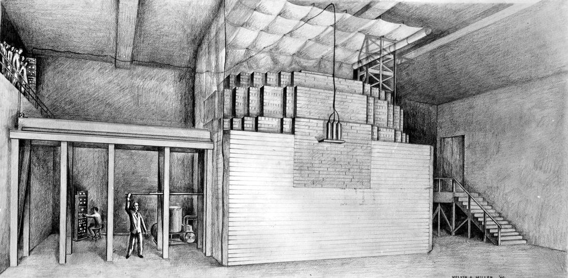
Back in the 1940s, Enrico Fermi started to wonder whether a self-sustained fission reaction was possible. So he and his team started to study how these brand-new particles discovered by James Chadwick and called neutrons behaved. And they found that neutrons are not deterministic but rather statistic in nature. They wander from here to there and they interact with nuclei more or less randomly, although the probabilities of different reactions are well-defined and can be measured. Having a significant amount (trillions) of neutrons greatly decreases the statistical variance so at the end of the day, deterministic calculations may be used. If you played one trillion hands of double-deck blackjack you would have gotten exactly 64/1339 \approx 4.7797\dots \% naturals. It was in this way (the variance reduction, not the cards) how Fermi was able to achieve criticality—a term which we will revisit below—in the Chicago Pile-1 using paper and pencil.
The Montecarlo method
A couple of years later, a number of people gathered together in New Mexico to work in a tiny little project code-named Manhattan. These guys started using Fermi’s neutron diffusion equation, but they soon realized that in some experiments they did not have enough neutrons to overcome the statistical variance. So Stanislaw Ulam developed a computation method based on tracking individual neutrons taking their statistical nature into account. Hence, the modern Montecarlo Method was born, named of course after the casino, that brings us back to blackjack somehow.
Remark #1 All those consultants that claim to perform “Montecarlo Calculations” ought to know that they borrowed that term from the nuclear industry.
Remark #2 All those startups that say “critical mass” to mean “a reasonable number of clients” ought to know that they borrowed that term also from the nuclear industry.
Remark #3 Luckily, the original Montecarlo Method was contemporary to the incipient development of electronic computers that allowed an efficient way of statistically modeling individual neutrons through their random paths.
Remark #4 Also lucky was the fact that the birth of the nuclear industry was a couple of years before the rise of the space exploration program, otherwise astronauts would have been fried by invisible and mysterious reasons (i.e. high-energy gamma radiation and sub-atomic charged particles).
Buffon’s needle
Long before neutrons, Count Buffon proved that if one has a long table of length L over which transversal lines separated by a length d are drawn and a stick (needle) of length \ell is randomly thrown over the table, then the probability p that the stick crosses one line is (for \ell < d)
p = \frac{ 2 \ell }{ \pi d }
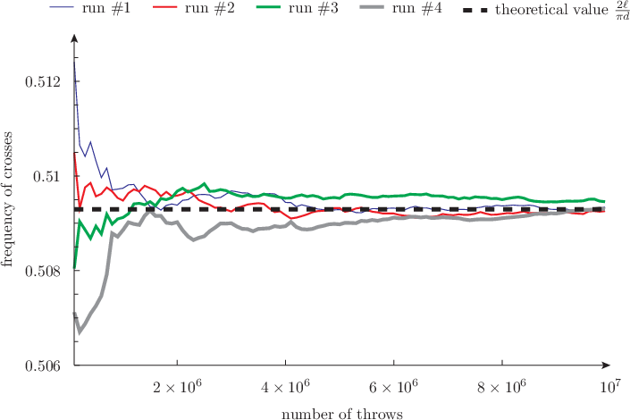
So, it is hard to avoid the temptation of grabbing a computer and start throwing (virtual) sticks over the table. Using wasora, we can simulate throwing a stick over the table as many times as we want:
VAR count           # number of times the stick crosses one line
static_steps = 1e7  # number of times we trow the stick

CONST L l d result

L = 10    # length of the table
l = 0.8   # length of the stick
d = 1     # distance between lines
result = 2*l/(pi*d) # expected theoretical result

x = random(0, L)          # location of the center of the stick
theta = random(0, 2*pi)   # the resulting angle

x1 = x + 0.5*l*cos(theta) # coordinates of the stick ends
x2 = x - 0.5*l*cos(theta)

# increase count if the stick crosses one line
# (remember ! is the "not equal" operator)
count = count + (floor(x1/d)!floor(x2/d))

# print the partial results
PRINT %g step_static count/step_static result SKIP_STATIC_STEP 1e5
See the Buffon’s needle problem in the wasora Real Book for further details.
This is the classical Montecarlo approach, and as such—getting into the main point of this article—it is a proper usage of the term “simulation.” Why? Because we are making a direct analogy between the physical act of throwing sticks over a table and taking sample from a pseudo-random number generator.3 We are “pretending” to do something we are not really doing (throwing sticks) with a mathematical analogy that lives inside a computer (taking a random number and pretending it is the location and angle of the thrown stick).
Mechanical analysis of a piston rod
Let us now switch our attention to the following problem. We have a mechanical part, say from the automotive industry, and we want to find out how it behaves under operational loads. We first start by getting the 3D CAD model (or building one ourselves using either FreeCAD or Onshape for example). Then we fire up a computational tool based on the finite element method, define the problem, create a mesh, run a solver and see the results.
To further illustrate my point, let us consider the CAEplex tutorial (which is the same as Simscale’s first tutorial):
Some people would say that this is a “virtual simulation” or even a “virtual experiment.”4 I beg to differ. I fail to see what the distribution of the Von Mises Stresses in the above connecting rod obtained as a result of a set of equations that contain many assumptions and idealizations (i.e. models that are beyond the scope of this opinion article) has to do with “simulation.” All we did was to solve a set of deterministic equations that are a variation of the ones proposed by Sir Isaac Newton mixed up with some mathematical models (i.e. Hooke’s law) and draw the results with colors. We have not faked anything. We have not pretended we did something we did not do.
Thermal modeling
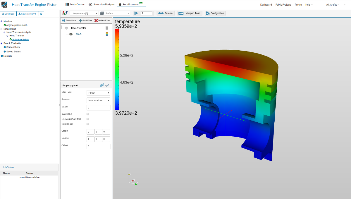
In a similar sense, in the following embed we can see the results of a thermal model of a piston head, not a simulation:
We already have visited this issue earlier this year by commenting an article by Ora Research regarding The Uber Cloud Experiment5:
Say “simulation” only if you are “simulating”
Of course you are free to say whatever you want to say. I am not as stubborn as RMS is. But let me propose the following helper table:
| Problem | Simulation | Modeling |
|---|---|---|
| Blackjack | LibreBlackjack | Blackjack Suite |
| Neutronics | Helios++ | milonga |
| Mechanics | – | z88, code_aster, XC |
| Thermal | – | Fino, CALCULIX |
| CFD | – | OpenFOAM, PETSc-FEM |
dnl Of course, whatever name you decide to call it, please always do use free and open source programs. Stay away from privative software—especially regarding engineering analysis—because it first takes away your freedom and then it prevents from understanding, sharing and modifying the equations that contain the models you are relying on.
There is a generalized idea that “FEA” (Finite-Element Analysis) means “structural analysis” whilst “CFD” (Computational Fluid Dynamics) means fluid mechanics problems. The latter is almost right, thought steady-state fluid problems fall into this category too. But the former is wrong, because the Finite Element Method is a general mathematical concept that may be used to solve a wide variety of partial differential equations, not just mechanical problems. It can even be used to solve CFD problems, although they are more prone to be solved using the finite volumes method. So enumerating FEA and CFD in the same level is a conceptual mistake that has (sadly) diffused through the community and is now a common usage.↩︎
We even discussed up to some extend in private emails the subject of this post.↩︎
Every software-based random number generator is deterministic, although the seed can have a lot of entropy. This one, however is based on nuclear physics (again) and gives true random numbers.↩︎
Back when I was a student I was studying chaotic natural convection loops and one of the teachers in charge of an optional subject (not an engineer) asked if I had performed “experiments.” I said “yes, I have built an actual loop.” And she replied “oh, but I mean with the computer”—implying that for her, performing an experiment meant numerically solving a set of differential equations.↩︎
This time, the word experiment is correctly employed, as it does not refer to “solving equations” but to performing an actual experiment, namely to evaluate the impact of shifting HPC to cloud-based infrastructures.↩︎
