NAFEMS LE10 thick plate pressure benchmark
← Previous: NAFEMS LE1 plane-stress benchmark | ↑ Index | Next: Stresses in a 10-node tetrahedron with prescribed displacements →
| Title | NAFEMS LE10 thick plate pressure benchmark |
| Tags | NAFEMS benchmark parametric |
| Runnng time | 0.1 sec |
| See also | 010-nafems-le1 |
| CAEplex case | https://caeplex.com/p/bc1bf |
| Available in | HTML PDF ePub |
1 Problem description
Consider the NAFEMS LE10 thick plate pressure benchmark problem from 1990, which belongs to The Standard NAFEMS Benchmarks. There are public solutions available online using a wide variety of FEA solvers such as this, this, this, this and this one. Do not hesitate contacting us if you want to add another reference to the list.
As shown in the original fig. 1, the problem consists of a thick plate defined by two ellipses. The plate is loaded on one of the plane surfaces with an uniform compression pressure p=1~\text{MPa}. Due to symmetry, only one quarter of the plate needs to be modeled with appropriate displacement conditions. The mid-plane edge of the outermost face is fixed in the load direction. Material’s Young modulus is E=210~\text{GPa} and Poisson’s ratio is \nu=0.3. The objective is to compute the normal stress in the y direction at the corner D=(2~\text{m},0~\text{m},0.6~\text{m}).

1.1 Expected results
The reference solution given in the original NAFEMS book is \sigma_y = -5.38~\text{MPa}.

2 Fino input file
In this case file, we start by showing the Fino input file that illustrates its design basis about the correlation of the almost-plain-English input file and the problem being solved. See how well this annotated input file le10.fin correlates to the original problem definition in fig. 1:
# NAFEMS Benchmark #10: thick plate pressure
# Reference solution: -5.38 MPa

MESH FILE_PATH le10.msh   # read the mesh

# loading
PHYSICAL_GROUP upper    BC p=-1     # uniform normal pressure of 1 MPa on the upper surface

# fixtures
PHYSICAL_GROUP DCD'C'   BC v=0      # Face DCD'C' zero y-displacement
PHYSICAL_GROUP ABA'B'   BC u=0      # Face ABA'B' zero x-displacement
PHYSICAL_GROUP BCB'C'   BC u=0 v=0  # Face BCB'C' x and y displ. fixed
PHYSICAL_GROUP midplane BC w=0      #  z displacemenrs fixed along mid-plane

# material properties
E = 210e3   # Young modulus in MPa
nu = 0.3    # Poisson’s ratio

FINO_STEP    # solve!

MESH_POST FILE_PATH le10.vtk VECTOR u v w sigmay    # write post-processing view in VTK

# write some (optional) information into the screen/terminal
PRINT "number of elements = " elements
PRINT "   number of nodes = " nodes
PRINT "   total wall time = " %.1f time_wall_total " secs"
PRINT "[u,v,w] @ D = [" u(2000,0,600) v(2000,0,600) w(2000,0,600) "] mm"   SEP " "
PRINT "sigma_y @ D = " sigmay(2000,0,600) "MPa"                            SEP " "
PRINT "  error @ D = " %.2f 100*abs(sigmay(2000,0,600)+5.38)/5.38 TEXT "%" SEP " "
3 Geometry and mesh
Both the geometry and the mesh are created in Gmsh using the OpenCASCADE kernel. This procedure is slightly more complex than what we saw in the previous section but it is because we build the CAD ourselves with actual ellipses using OpenCASCADE. Then we ask Gmsh to use 20-node hexahedra to create a 6 \times 4 \times 2 structured grid—just as the original problem suggests—with the following le10.geo Gmsh script:
// NAFEMS LE10 benchmark geometry & mesh
SetFactory("OpenCASCADE");

a = 1000;   // geometric parameters (in mm)
b = 2750;
c = 3250;
d = 2000;
h = 600;

Point(1) = {0, a, 0};  // define the four points A, B, C and D
Point(2) = {0, b, 0};
Point(3) = {c, 0, 0};
Point(4) = {d, 0, 0};


Line(1) = {1, 2};      // join them with the ellipses and straight edges
Ellipse (2) = {0,0,0, c, b, 0, Pi/2};
Line(3) = {3, 4};
Ellipse (4) = {0,0,0, d, a, 0, Pi/2};
Coherence;             // merge the points

Curve Loop(1) = {1, -2, 3, 4};   // create the bottom surface
Plane Surface(1) = {1};

Extrude {0, 0, 0.5*h} { Surface{1}; }   // extrude it (twice to get the mid-plane edge)
Extrude {0, 0, 0.5*h} { Surface{6}; }

Physical Surface("DCD'C'") = {9, 4};    // define physical groups for boundary conditions
Physical Surface("ABA'B'") = {7, 2};
Physical Surface("BCB'C'") = {8, 3};
Physical Surface("upper") = {11};
Physical Curve("midplane") = {9};
Physical Volume("bulk") = {1,2};

// meshing settings
Mesh.ElementOrder = 2;          // use second-order
Mesh.RecombineAll = 1;          // use hexas instead of tets
Mesh.SecondOrderLinear = 0;     // use curved elemetns
Mesh.SecondOrderIncomplete = 1; // use hex20 instead of hex27

// ask for a structured mesh
// the original 6x4x2 NAFEMS "fine" mesh is obtained with CharacteristicLengthFactor = 1
Transfinite Curve{2,9,17,4,12,20} = 6/Mesh.CharacteristicLengthFactor + 1;
Transfinite Curve{1,7,15,3,11,19} = 4/Mesh.CharacteristicLengthFactor + 1;
Transfinite Curve{5,13,6,14,8,16,10,18} = 1/Mesh.CharacteristicLengthFactor + 1;
Transfinite Surface {1,2,3,4,5,6,7,8,9,10,11};
Transfinite Volume {1,2};
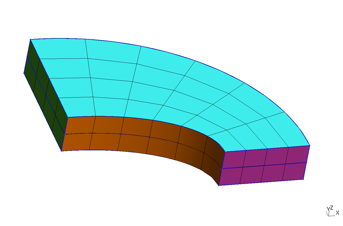
Figure 2: Hexahedral meshes for the NAFEMS LE10 benchmark problem.. a — The “official” 1990 meshes., b — 6 \times 4 \times 2 20-node hexahedra structured mesh created by Gmsh.
4 Execution
First Gmsh is invoked to create the mesh le10.msh out of le10.geo and then Fino is instructed to read le10.fin:
$ gmsh -3 le10.geo
[...]
$ fino le1-base.fin
number of elements =    106
   number of nodes =    349
   total wall time =    0.1      secs
[u,v,w] @ D = [ -0.0276353 -1.2544e-08 -0.098182 ] mm
sigma_y @ D =  -5.36013 MPa
  error @ D =  0.37 %
$
5 Results
The output file le10.vtk created by Fino can be post-processed with ParaView as shown in fig. 3
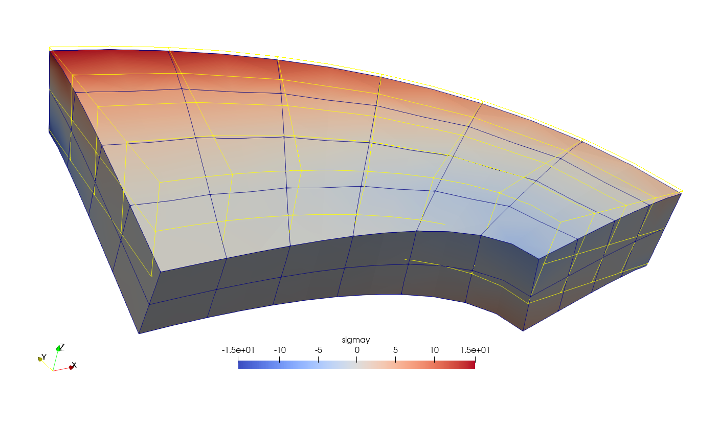
5.1 Check
The normal stress is pretty close to the reference value \sigma_y = -5.38~\text{MPa}. What about finer grids?
$ gmsh -3 le10.geo -clscale 0.2
[...]
$ fino le10.fin
number of elements =    7330
   number of nodes =    27421
   total wall time =    13.5     secs
[u,v,w] @ D = [ -0.0275038 -1.21177e-09 -0.102571 ] mm
sigma_y @ D =  -5.40646 MPa
  error @ D =  0.49 %
$
So more nodes take us “away” from the target. Let’s refine further…
$ gmsh -3 le10.geo -clscale 0.15
[...]
$ fino le10.fin
number of elements =    14664
   number of nodes =    55573
   total wall time =    28.2     secs
[u,v,w] @ D = [ -0.0275132 3.86036e-09 -0.103191 ] mm
sigma_y @ D =  -5.39536 MPa
  error @ D =  0.29 %
$
Now we are back on the track!. A little bit further…
$ gmsh -3 le10.geo -clscale 0.11
[...]
$ fino le10.fin
number of elements =    39258
   number of nodes =    150877
   total wall time =    77.4     secs
[u,v,w] @ D = [ -0.0275247 7.79166e-10 -0.104186 ] mm
sigma_y @ D =  -5.38217 MPa
  error @ D =  0.04 %
$
One more…
$ gmsh -3 le10.geo -clscale 0.10
[...]
$ fino le10.fin
number of elements =    53260
   number of nodes =    205441
   total wall time =    108.6    secs
[u,v,w] @ D = [ -0.0275284 4.38467e-09 -0.104476 ] mm
sigma_y @ D =  -5.37908 MPa
  error @ D =  0.02 %
$
and there you go! We made it “to the other side.”
Note that we used the very same Fino input file
le10.finfor all the cases. We only needed to ask Gmsh to use a different element length scaling factor through its command-line argument-clscaleand that was it.
6 Mesh convergence
Can we study the convergence in a less “artisanal” way and use some systematic and repeatable scheme? Sure thing! Fino’s (actually wasora’s) keyword PARAMETRIC comes in.
# sweep n = mesh refinement factor
DEFAULT_ARGUMENT_VALUE 1 hex20
DEFAULT_ARGUMENT_VALUE 2 struct
DEFAULT_ARGUMENT_VALUE 3 curved
DEFAULT_ARGUMENT_VALUE 4 5
PARAMETRIC n MIN 1 MAX $4 STEP 1

# call gmsh to compute mesh(n)
SHELL "gmsh -v 0 -3 le10-base.geo $1.geo $2.geo $3.geo -clscale %g -o le10-$1-$2-$3-%g.msh" 1/n n

# read it back
INPUT_FILE mesh le10-$1-$2-$3-%g.msh n
MESH FILE mesh

E = 210e3   # [ MPa ]
nu = 0.3

# fixtures
PHYSICAL_GROUP DCD'C'   BC v=0
PHYSICAL_GROUP ABA'B'   BC u=0
PHYSICAL_GROUP BCB'C'   BC u=0 v=0
PHYSICAL_GROUP midplane BC w=0

# load
PHYSICAL_GROUP upper    BC p=-1

FINO_STEP   # solve!

PRINT 3*nodes sigmay(2000,0,600) u(2000,0,600) v(2000,0,600) w(2000,0,600) time_wall_total memory/1024