1 Overview
2 Introduction
3 Running feenox
- 3.1 Invocation
- 3.2 Compilation
4 Examples
5 Tutorials
6 Description
7 Reference
8 FeenoX & the Unix Philospohy
9 History

1 Overview

FeenoX is a computational tool that can solve engineering problems which are usually casted as differential-algebraic equations (DAEs) or partial differential equations (PDEs). It is to finite elements programs and libraries what Markdown is to Word and TeX, respectively. In particular, it can solve

dynamical systems defined by a set of user-provided DAEs (such as plant control dynamics for example)
mechanical elasticity
heat conduction
structural modal analysis
neutron diffusion
neutron transport

FeenoX reads a plain-text input file which contains the problem definition and writes 100%-user defined results in ASCII (through PRINT or other user-defined output instructions within the input file). For PDE problems, it needs a reference to at least one Gmsh mesh file for the discretization of the domain. It can write post-processing views in either .msh or .vtk formats.

Keep in mind that FeenoX is just a back end reading a set of input files and writing a set of output files following the design philosophy of Unix (separation, composition, representation, economy, extensibility, etc). Think of it as a transfer function (or a filter in computer-science jargon) between input files and output files:

                             +------------+
 mesh (*.msh)  }             |            |             { terminal
 data (*.dat)  } input ----> |   FeenoX   |----> output { data files
 input (*.fee) }             |            |             { post (vtk/msh)
                             +------------+

Following the Unix programming philosophy, there are no graphical interfaces attached to the FeenoX core, although a wide variety of pre and post-processors can be used with FeenoX. To illustrate the transfer-function approach, consider the following input file that solves Laplace’s equation \nabla^2 \phi = 0 on a square with some space-dependent boundary conditions:

\begin{cases} \phi(x,y) = +y & \text{for $x=-1$ (left)} \\ \phi(x,y) = -y & \text{for $x=+1$ (right)} \\ \nabla \phi \cdot \hat{\vec{n}} = \sin\left(\frac{\pi}{2} \cdot x\right) & \text{for $y=-1$ (bottom)} \\ \nabla \phi \cdot \hat{\vec{n}} =0 & \text{for $y=+1$ (top)} \\ \end{cases}

PROBLEM laplace 2d
READ_MESH square-centered.msh # [-1:+1]x[-1:+1]

# boundary conditions
BC left    phi=+y
BC right   phi=-y
BC bottom  dphidn=sin(pi/2*x)
BC top     dphidn=0

SOLVE_PROBLEM

# same output in .msh and in .vtk formats
WRITE_MESH laplace-square.msh phi VECTOR dphidx dphidy 0
WRITE_MESH laplace-square.vtk phi VECTOR dphidx dphidy 0

Figure 1: Laplace’s equation solved with FeenoX. a — Post-processed with Gmsh, b — Post-processed with Paraview

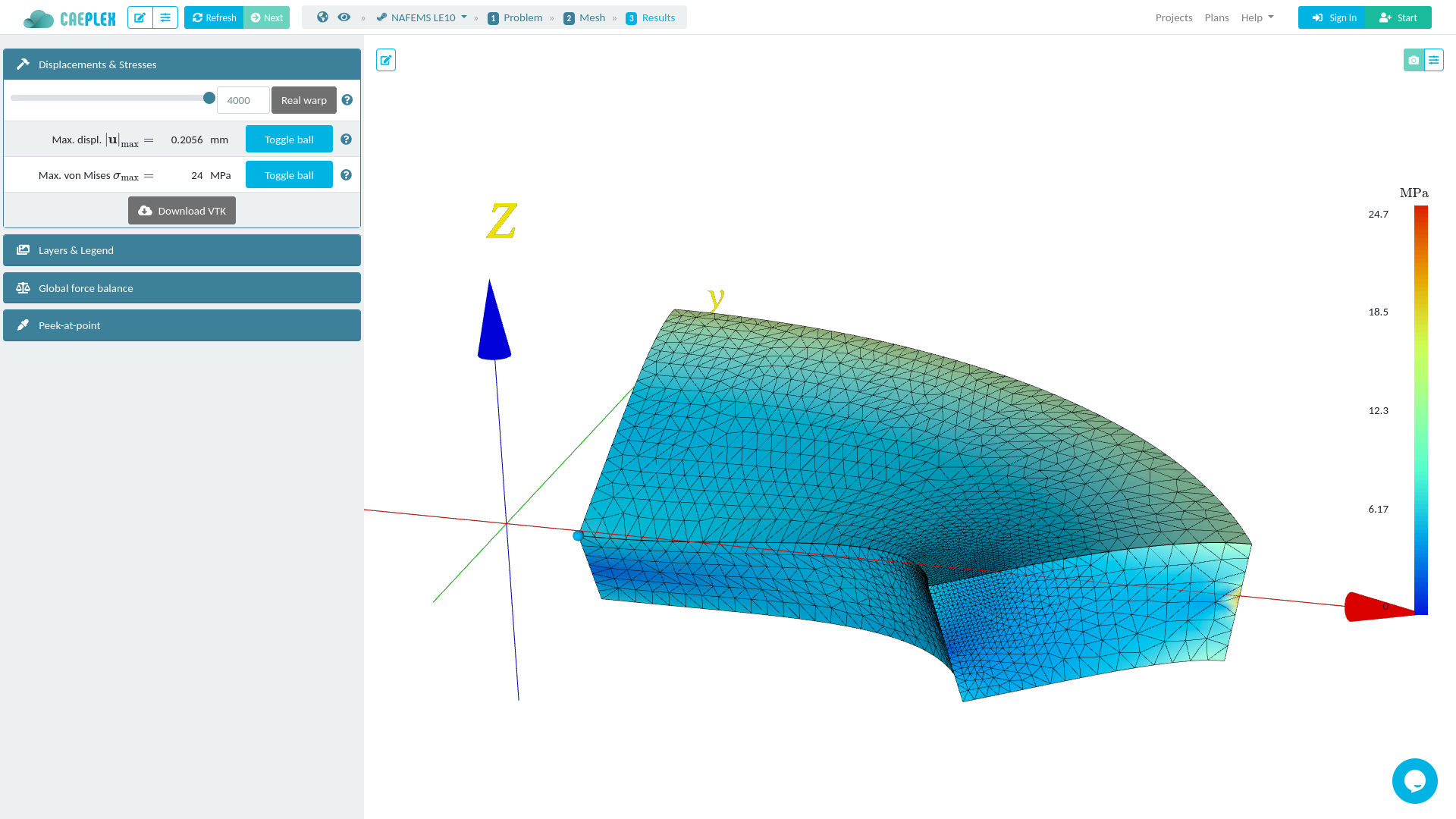
The .msh file can be post-processed with Gmsh, and the .vtk file can be post-processed with Paraview. See https://www.caeplex.com for a mobile-friendly web-based interface for solving finite elements in the cloud directly from the browser.

2 Introduction

FeenoX can be seen either as

a syntactically-sweetened way of asking the computer to solve engineering-related mathematical problems, and/or
a finite-element(ish) tool with a particular design basis.

Note that some of the problems solved with FeenoX might not actually rely on the finite element method, but on general mathematical models and even on the finite volumes method. That is why we say it is a finite-element(ish) tool.

In other words, FeenoX is a computational tool to solve

dynamical systems written as sets of ODEs/DAEs, or
steady or transient heat conduction problems, or
steady or quasi-static thermo-mechanical problems, or
modal analysis problems, or
core-level steady-state neutronics, or
community-contributed problems

in such a way that the input is a near-English text file that defines the problem to be solved.

One of the main features of this allegedly particular design basis is that simple problems ought to have simple inputs (rule of simplicity) or, quoting Alan Kay, “simple things should be simple, complex things should be possible.”

For instance, to solve one-dimensional heat conduction over the domain x\in[0,1] (which is indeed one of the most simple engineering problems we can find) the following input file is enough:

PROBLEM thermal 1D               # tell FeenoX what we want to solve 
READ_MESH slab.msh               # read mesh in Gmsh's v4.1 format
k = 1                            # set uniform conductivity
BC left  T=0                     # set fixed temperatures as BCs
BC right T=1                     # "left" and "right" are defined in the mesh
SOLVE_PROBLEM                    # tell FeenoX we are ready to solve the problem
PRINT T(0.5)                     # ask for the temperature at x=0.5

$ feenox thermal-1d-dirichlet-constant-k.fee 
0.5
$

The mesh is assumed to have been already created with Gmsh (or any other pre-processing tool and converted to .msh format with Meshio for example). This assumption follows the rule of composition and prevents the actual input file from being polluted with mesh-dependent data (such as node coordinates and/or nodal loads) so as to keep it simple and make it Git-friendly (rule of generation). The only link between the mesh and the FeenoX input file is through physical groups (in the case above left and right) used to set boundary conditions and/or material properties.

Another design-basis decision is that similar problems ought to have similar inputs (rule of least surprise). So in order to have a space-dependent conductivity, we only have to replace one line in the input above: instead of defining a scalar k we define a function of x (we also update the output to show the analytical solution as well):

PROBLEM thermal 1D
READ_MESH slab.msh
k(x) = 1+x                       # space-dependent conductivity
BC left  T=0
BC right T=1
SOLVE_PROBLEM
PRINT T(1/2) log(1+1/2)/log(2)   # print numerical and analytical solutions

$ feenox thermal-1d-dirichlet-space-k.fee 
0.584959	0.584963
$

The other main decision in FeenoX design is an everything is an expression design principle, meaning that any numerical input can be an algebraic expression (e.g. T(1/2) is the same as T(0.5)). If we want to have a temperature-dependent conductivity (which renders the problem non-linear) we can take advantage of the fact that T(x) is available not only as an argument to PRINT but also for the definition of algebraic functions:

PROBLEM thermal 1D
READ_MESH slab.msh
k(x) = 1+T(x)                    # temperature-dependent conductivity
BC left  T=0
BC right T=1
SOLVE_PROBLEM
PRINT T(1/2) sqrt(1+(3*0.5))-1   # print numerical and analytical solutions

$ feenox thermal-1d-dirichlet-temperature-k.fee 
0.581139	0.581139
$

Let us consider the famous chaotic Lorenz’s dynamical system. Here is one way of getting an image of the butterfly-shaped attractor using FeenoX to compute it and Gnuplot to draw it. Solve

\begin{cases} \dot{x} &= \sigma \cdot (y - x) \\ \dot{y} &= x \cdot (r - z) - y \\ \dot{z} &= x y - b z \\ \end{cases}

for 0 < t < 40 with initial conditions

\begin{cases} x(0) = -11 \\ y(0) = -16 \\ z(0) = 22.5 \\ \end{cases}

and \sigma=10, r=28 and b=8/3, which are the classical parameters that generate the butterfly as presented by Edward Lorenz back in his seminal 1963 paper Deterministic non-periodic flow.

The following ASCII input file ressembles the parameters, inital conditions and differential equations of the problem as naturally as possible:

PHASE_SPACE x y z     # Lorenz attractor’s phase space is x-y-z
end_time = 40         # we go from t=0 to 40 non-dimensional units

sigma = 10            # the original parameters from the 1963 paper
r = 28
b = 8/3

x_0 = -11             # initial conditions
y_0 = -16
z_0 = 22.5

# the dynamical system's equations written as naturally as possible
x_dot = sigma*(y - x)
y_dot = x*(r - z) - y
z_dot = x*y - b*z

PRINT t x y z        # four-column plain-ASCII output

Figure 2: The Lorenz attractor solved with FeenoX and drawn with Gnuplot

Indeed, when executing FeenoX with this input file, we get four ASCII columns (t, x, y and z) which we can then redirect to a file and plot it with a standard tool such as Gnuplot. Note the importance of relying on plain ASCII text formats both for input and output, as recommended by the Unix philosophy and the rule of composition: other programs can easily create inputs for FeenoX and other programs can easily understand FeenoX’s outputs. This is essentially how Unix filters and pipes work.

Note the one-to-one correspondence between the human-friendly differential equations (written in TeX and rendered as typesetted mathematical symbols) and the computer-friendly input file that FeenoX reads.

Let us solve the linear elasticity benchmark problem NAFEMS LE10 “Thick plate pressure.” with FeenoX. Note the one-to-one correspondence between the human-friendly problem statement from fig. 3 and the FeenoX input file:

Figure 3: The NAFEMS LE10 problem statement and the corresponding FeenoX input

# NAFEMS Benchmark LE-10: thick plate pressure
PROBLEM mechanical DIMENSIONS 3
READ_MESH nafems-le10.msh   # mesh in millimeters

# LOADING: uniform normal pressure on the upper surface
BC upper    p=1      # 1 Mpa

# BOUNDARY CONDITIONS:
BC DCD'C'   v=0      # Face DCD'C' zero y-displacement
BC ABA'B'   u=0      # Face ABA'B' zero x-displacement
BC BCB'C'   u=0 v=0  # Face BCB'C' x and y displ. fixed
BC midplane w=0      #  z displacements fixed along mid-plane

# MATERIAL PROPERTIES: isotropic single-material properties
E = 210e3   # Young modulus in MPa
nu = 0.3    # Poisson's ratio

SOLVE_PROBLEM   # solve!

# print the direct stress y at D (and nothing more)
PRINT "σ_y @ D = " sigmay(2000,0,300) "MPa"

Here, “one-to-one” means that the input file does not need any extra definition which is not part of the problem formulation. Of course the cognizant engineer can give further definitions such as

the linear solver and pre-conditioner
the tolerances for iterative solvers
options for computing stresses out of displacements
etc.

However, she is not obliged to as–at least for simple problems—the defaults are reasonable. This is akin to writing a text in Markdown where one does not need to care if the page is A4 or letter (as, in most cases, the output will not be printed but rendered in a web browser).

The problem asks for the normal stress in the y direction \sigma_y at point “D,” which is what FeenoX writes (and nothing else, rule of economy):

$ feenox nafems-le10.fee 
sigma_y @ D =   -5.38016        MPa
$

Also note that since there is only one material, there is no need to do an explicit link between material properties and physical volumes in the mesh (rule of simplicity). And since the properties are uniform and isotropic, a single global scalar for E and a global single scalar for \nu are enough.

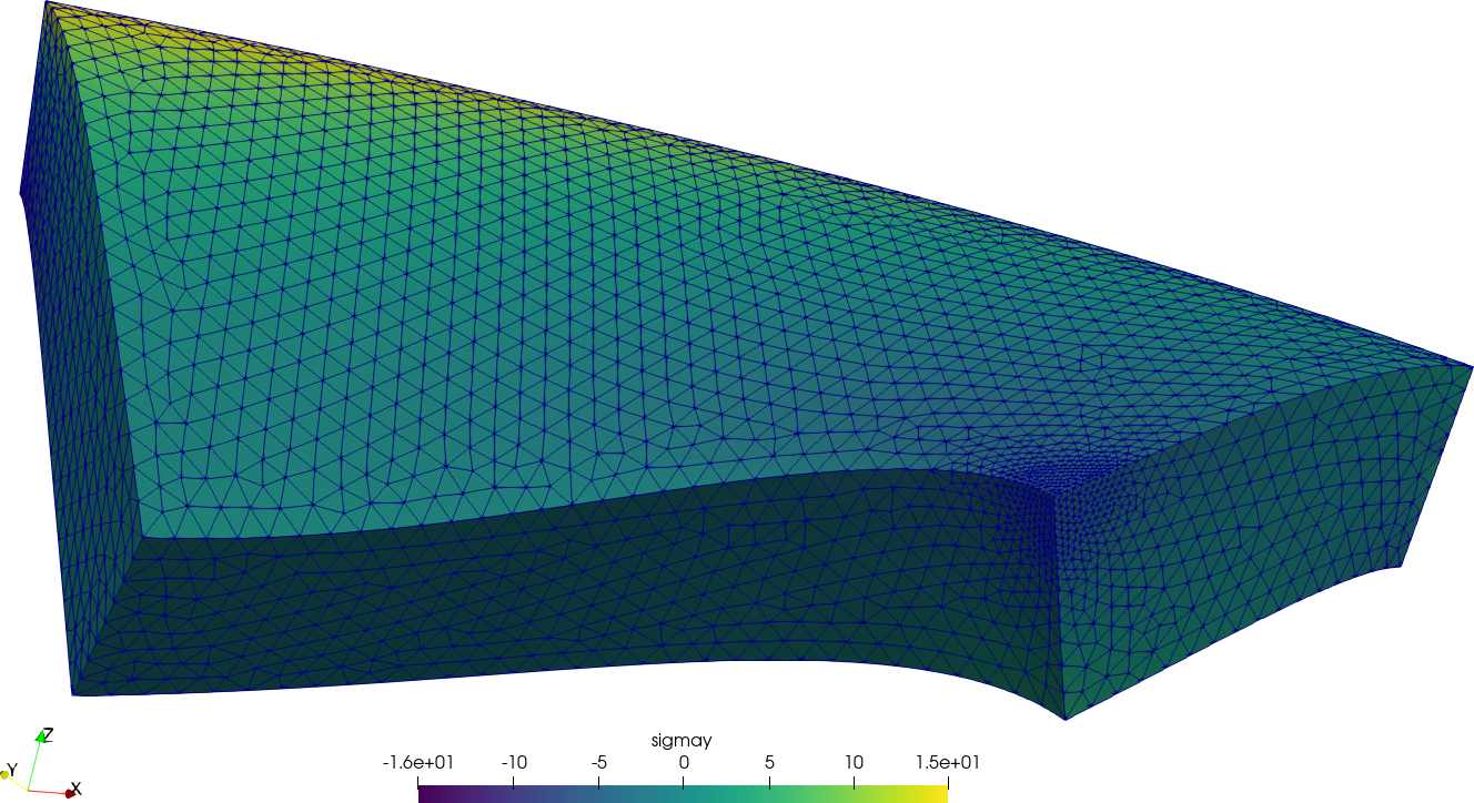
Figure 4: Normal stress \sigma_y refined around point D over 5,000x-warped displacements for LE10 created with Paraview

For the sake of visual completeness, post-processing data with the scalar distribution of \sigma_y and the vector field of displacements [u,v,w] can be created by adding one line to the input file:

WRITE_MESH nafems-le10.vtk sigmay VECTOR u v w

This VTK file can then be post-processed to create interactive 3D views, still screenshots, browser and mobile-friendly webGL models, etc. In particular, using Paraview one can get a colorful bitmapped PNG (the displacements are far more interesting than the stresses in this problem).

Figure 5: See also https://caeplex.com/r/f1a82f to see this very same LE10 problem solved in the mobile-friendly web-based interface CAEplex that uses FeenoX as the back end

Please note the following two points about both cases above:

The input files are very similar to the statements of each problem in plain English words (rule of clarity). Those with some experience may want to compare them to the inputs decks (sic) needed for other common FEA programs.
By design, 100% of FeenoX’s output is controlled by the user. Had there not been any PRINT or WRITE_MESH instructions, the output would have been empty, following the rule of silence. This is a significant change with respect to traditional engineering codes that date back from times when one CPU hour was worth dozens (or even hundreds) of engineering hours. At that time, cognizant engineers had to dig into thousands of lines of data to search for a single individual result. Nowadays, following the rule of economy, it is actually far easier to ask the code to write only what is needed in the particular format that suits the user.

Some basic rules are

FeenoX is just a solver working as a transfer function between input and output files.

                             +------------+
 mesh (*.msh)  }             |            |             { terminal
 data (*.dat)  } input ----> |   FeenoX   |----> output { data files
 input (*.fee) }             |            |             { post (vtk/msh)
                             +------------+

Following the rules of separation, parsimony and diversity, there is no embedded graphical interface but means of using generic pre and post processing tools—in particular, Gmsh and Paraview respectively. See also CAEplex for a web-based interface.

The input files should be syntactically sugared so as to be as self-describing as possible.
Simple problems ought to need simple input files.
Similar problems ought to need similar input files.
Everything is an expression. Whenever a number is expected, an algebraic expression can be entered as well. Variables, vectors, matrices and functions are supported. Here is how to replace the boundary condition on the right side of the slab above with a radiation condition:
```
sigma = 1       # non-dimensional stefan-boltzmann constant
e = 0.8         # emissivity 
Tinf=1          # non-dimensional reference temperature
BC right q=sigma*e*(Tinf^4-T(x)^4)
```
This “everything is an expression” principle directly allows the application of the Method of Manufactured Solutions for code verification.
FeenoX should run natively in the cloud and be able to massively scale in parallel. See the Software Requirements Specificationa> and the Software Development Specification for details.

Since it is free (as in freedom) and open source, contributions to add features (and to fix bugs) are welcome. In particular, each kind of problem supported by FeenoX (thermal, mechanical, modal, etc.) has a subdirectory of source files which can be used as a template to add new problems, as implied in the “community-contributed problems” bullet above (rules of modularity and extensibility). See the documentation for details about how to contribute.

3 Running `feenox`

3.1 Invocation

The format for running the feenox program is:

feenox [options] inputfile [optional_extra_arguments] ...

The feenox executable supports the following options:

feenox [options] inputfile [replacement arguments] [petsc options]

-h, --help: display options and detailed explanations of commmand-line usage
-v, --version: display brief version information and exit
-V, --versions: display detailed version information
-c, --check: validates if the input file is sane or not
--pdes: list the types of PROBLEMs that FeenoX can solve, one per line
--elements_info: output a document with information about the supported element types
--linear: force FeenoX to solve the PDE problem as linear
--non-linear: force FeenoX to solve the PDE problem as non-linear
--progress: print ASCII progress bars when solving PDEs
--mumps: ask PETSc to use the direct linear solver MUMPS

Instructions will be read from standard input if “-” is passed as inputfile, i.e.

$ echo 'PRINT 2+2' | feenox -
4

The optional [replacement arguments] part of the command line mean that each argument after the input file that does not start with an hyphen will be expanded verbatim in the input file in each occurrence of $1, $2, etc. For example

$ echo 'PRINT $1+$2' | feenox - 3 4
7

PETSc and SLEPc options can be passed in [petsc options] (or [options]) as well, with the difference that two hyphens have to be used instead of only once. For example, to pass the PETSc option -ksp_view the actual FeenoX invocation should be

$ feenox input.fee --ksp_view

For PETSc options that take values, en equal sign has to be used:

$ feenox input.fee --mg_levels_pc_type=sor

See https://www.seamplex.com/feenox/examples for annotated examples.

3.2 Compilation

These detailed compilation instructions are aimed at amd64 Debian-based GNU/Linux distributions. The compilation procedure follows the POSIX standard, so it should work in other operating systems and architectures as well. Distributions not using apt for packages (i.e. yum) should change the package installation commands (and possibly the package names). The instructions should also work for in MacOS, although the apt-get commands should be replaced by brew or similar. Same for Windows under Cygwin, the packages should be installed through the Cygwin installer. WSL was not tested, but should work as well.

3.2.1 Quickstart

Note that the quickest way to get started is to download an already-compiled statically-linked binary executable. Note that getting a binary is the quickest and easiest way to go but it is the less flexible one. Mind the following instructions if a binary-only option is not suitable for your workflow and/or you do need to compile the source code from scratch.

On a GNU/Linux box (preferably Debian-based), follow these quick steps. See sec. 3.2.2 for the actual detailed explanations.

To compile the Git repository, proceed as follows. This procedure does need git and autoconf but new versions can be pulled and recompiled easily. If something goes wrong and you get an error, do not hesitate to ask in FeenoX’s discussion page.

Install mandatory dependencies
```
sudo apt-get update
sudo apt-get install gcc make git automake autoconf libgsl-dev
```
If you cannot install libgsl-dev but still have git and the build toolchain, you can have the configure script to download and compile it for you. See point 4 below.
Install optional dependencies (of course these are optional but recommended)
```
sudo apt-get install libsundials-dev petsc-dev slepc-dev
```

Clone Github repository

git clone https://github.com/seamplex/feenox

Boostrap, configure, compile & make
```
cd feenox
./autogen.sh
./configure
make -j4
```
If you cannot (or do not want to) use libgsl-dev from a package repository, call configure with --enable-download-gsl:
```
./configure --enable-download-gsl
```
If you do not have Internet access, get the tarball manually, copy it to the same directory as configure and run again. See the detailed compilation instructions for an explanation.
Run test suite (optional)
```
make check
```
Install the binary system wide (optional)
```
sudo make install
```

To stay up to date, pull and then autogen, configure and make (and optionally install):

git pull
./autogen.sh; ./configure; make -j4
sudo make install

3.2.2 Detailed configuration and compilation

The main target and development environment is Debian GNU/Linux, although it should be possible to compile FeenoX in any free GNU/Linux variant (and even the in non-free MacOS and/or Windows platforms) running in virtually any hardware platform. FeenoX can run be run either in HPC cloud servers or a Raspberry Pi, and almost everything that sits in the middle.

Following the Unix philosophy discussed in the SDS, FeenoX re-uses a lot of already-existing high-quality free and open source libraries that implement a wide variety of mathematical operations. This leads to a number of dependencies that FeenoX needs in order to implement certain features.

There is only one dependency that is mandatory, namely GNU GSL (see sec. 3.2.2.1.1), which if it not found then FeenoX cannot be compiled. All other dependencies are optional, meaning that FeenoX can be compiled but its capabilities will be partially reduced.

As per the SRS, all dependencies have to be available on mainstream GNU/Linux distributions and have to be free and open source software. But they can also be compiled from source in case the package repositories are not available or customized compilation flags are needed (i.e. optimization or debugging settings).

In particular, PETSc (and SLEPc) also depend on other mathematical libraries to perform particular operations such as low-level linear algebra operations. These extra dependencies can be either free (such as LAPACK) or non-free (such as Intel’s MKL), but there is always at least one combination of a working setup that involves only free and open source software which is compatible with FeenoX licensing terms (GPLv3+). See the documentation of each package for licensing details.

3.2.2.1 Mandatory dependencies

FeenoX has one mandatory dependency for run-time execution and the standard build toolchain for compilation. It is written in C99 so only a C compiler is needed, although make is also required. Free and open source compilers are favored. The usual C compiler is gcc but clang or Intel’s icc and the newer icx can also be used.

Note that there is no need to have a Fortran nor a C++ compiler to build FeenoX. They might be needed to build other dependencies (such as PETSc and its dependencies), but not to compile FeenoX if all the dependencies are installed from the oeprating system’s package repositories. In case the build toolchain is not already installed, do so with

sudo apt-get install gcc make

If the source is to be fetched from the Git repository then not only is git needed but also autoconf and automake since the configure script is not stored in the Git repository but the autogen.sh script that bootstraps the tree and creates it. So if instead of compiling a source tarball one wants to clone from GitHub, these packages are also mandatory:

sudo apt-get install git automake autoconf

Again, chances are that any existing GNU/Linux box has all these tools already installed.

3.2.2.1.1 The GNU Scientific Library

The only run-time dependency is GNU GSL (not to be confused with Microsoft GSL). It can be installed with

sudo apt-get install libgsl-dev

In case this package is not available or you do not have enough permissions to install system-wide packages, there are two options.

Pass the option --enable-download-gsl to the configure script below.
Manually download, compile and install GNU GSL

If the configure script cannot find both the headers and the actual library, it will refuse to proceed. Note that the FeenoX binaries already contain a static version of the GSL so it is not needed to have it installed in order to run the statically-linked binaries.

3.2.2.2 Optional dependencies

FeenoX has three optional run-time dependencies. It can be compiled without any of these, but functionality will be reduced:

SUNDIALS provides support for solving systems of ordinary differential equations (ODEs) or differential-algebraic equations (DAEs). This dependency is needed when running inputs with the PHASE_SPACE keyword.
PETSc provides support for solving partial differential equations (PDEs). This dependency is needed when running inputs with the PROBLEM keyword.
SLEPc provides support for solving eigen-value problems in partial differential equations (PDEs). This dependency is needed for inputs with PROBLEM types with eigen-value formulations such as modal and neutron_sn.

In absence of all these, FeenoX can still be used to

solve general mathematical problems such as the ones to compute the Fibonacci sequence or the Logistic map,
operate on functions, either algebraically or point-wise interpolated such as Computing the derivative of a function as a Unix filter
read, operate over and write meshes,
etc.

These optional dependencies have to be installed separately. There is no option to have configure to download them as with --enable-download-gsl. When running the test suite (sec. 3.2.2.6), those tests that need an optional dependency which was not found at compile time will be skipped.

3.2.2.2.1 SUNDIALS

SUNDIALS is a SUite of Nonlinear and DIfferential/ALgebraic equation Solvers. It is used by FeenoX to solve dynamical systems casted as DAEs with the keyword PHASE_SPACE, like the Lorenz system.

Install either by doing

sudo apt-get install libsundials-dev

or by following the instructions in the documentation.

3.2.2.2.2 PETSc

The Portable, Extensible Toolkit for Scientific Computation, pronounced PET-see (/ˈpɛt-siː/), is a suite of data structures and routines for the scalable (parallel) solution of scientific applications modeled by partial differential equations. It is used by FeenoX to solve PDEs with the keyword PROBLEM, like the NAFEMS LE10 benchmark problem.

Install either by doing

sudo apt-get install petsc-dev

or by following the instructions in the documentation.

Note that

Configuring and compiling PETSc from scratch might be difficult the first time. It has a lot of dependencies and options. Read the official documentation for a detailed explanation.
There is a huge difference in efficiency between using PETSc compiled with debugging symbols and with optimization flags. Make sure to configure --with-debugging=0 for FeenoX production runs and leave the debugging symbols (which is the default) for development and debugging only.
FeenoX needs PETSc to be configured with real double-precision scalars. It will compile but will complain at run-time when using complex and/or single or quad-precision scalars.
FeenoX honors the PETSC_DIR and PETSC_ARCH environment variables when executing configure. If these two do not exist or are empty, it will try to use the default system-wide locations (i.e. the petsc-dev package).

3.2.2.2.3 SLEPc

The Scalable Library for Eigenvalue Problem Computations, is a software library for the solution of large scale sparse eigenvalue problems on parallel computers. It is used by FeenoX to solve PDEs with the keyword PROBLEM that need eigen-value computations, such as modal analysis of a cantilevered beam.

Install either by doing

sudo apt-get install slepc-dev

or by following the instructions in the documentation.

Note that

SLEPc is an extension of PETSc so the latter has to be already installed and configured.
FeenoX honors the SLEPC_DIR environment variable when executing configure. If it does not exist or is empty it will try to use the default system-wide locations (i.e. the slepc-dev package).
If PETSc was configured with --download-slepc then the SLEPC_DIR variable has to be set to the directory inside PETSC_DIR where SLEPc was cloned and compiled.

3.2.2.3 FeenoX source code

There are two ways of getting FeenoX’s source code:

Cloning the GitHub repository at https://github.com/seamplex/feenox
Downloading a source tarball from https://seamplex.com/feenox/dist/src/

3.2.2.3.1 Git repository

The main Git repository is hosted on GitHub at https://github.com/seamplex/feenox. It is public so it can be cloned either through HTTPS or SSH without needing any particular credentials. It can also be forked freely. See the Programming Guide for details about pull requests and/or write access to the main repository.

Ideally, the main branch should have a usable snapshot. All other branches can contain code that might not compile or might not run or might not be tested. If you find a commit in the main branch that does not pass the tests, please report it in the issue tracker ASAP.

After cloning the repository

git clone https://github.com/seamplex/feenox

the autogen.sh script has to be called to bootstrap the working tree, since the configure script is not stored in the repository but created from configure.ac (which is in the repository) by autogen.sh.

Similarly, after updating the working tree with

git pull

it is recommended to re-run the autogen.sh script. It will do a make clean and re-compute the version string.

3.2.2.3.2 Source tarballs

When downloading a source tarball, there is no need to run autogen.sh since the configure script is already included in the tarball. This method cannot update the working tree. For each new FeenoX release, the whole source tarball has to be downloaded again.

3.2.2.4 Configuration

To create a proper Makefile for the particular architecture, dependencies and compilation options, the script configure has to be executed. This procedure follows the GNU Coding Standards.

./configure

Without any particular options, configure will check if the mandatory GNU Scientific Library is available (both its headers and run-time library). If it is not, then the option --enable-download-gsl can be used. This option will try to use wget (which should be installed) to download a source tarball, uncompress, configure and compile it. If these steps are successful, this GSL will be statically linked into the resulting FeenoX executable. If there is no internet connection, the configure script will say that the download failed. In that case, get the indicated tarball file manually, copy it into the current directory and re-run ./configure.

The script will also check for the availability of optional dependencies. At the end of the execution, a summary of what was found (or not) is printed in the standard output:

$ ./configure
[...]
## ----------------------- ##
## Summary of dependencies ##
## ----------------------- ##
  GNU Scientific Library  from system
  SUNDIALS IDA            yes
  PETSc                   yes /usr/lib/petsc 
  SLEPc                   no
[...]

If for some reason one of the optional dependencies is available but FeenoX should not use it, then pass --without-sundials, --without-petsc and/or --without-slepc as arguments. For example

$ ./configure --without-sundials --without-petsc
[...]
## ----------------------- ##
## Summary of dependencies ##
## ----------------------- ##
  GNU Scientific Library  from system
  SUNDIALS                no
  PETSc                   no
  SLEPc                   no
[...]

If configure complains about contradicting values from the cached ones, run autogen.sh again before configure and/or clone/uncompress the source tarball in a fresh location.

To see all the available options run

./configure --help

3.2.2.5 Source code compilation

After the successful execution of configure, a Makefile is created. To compile FeenoX, just execute

make

Compilation should take a dozen of seconds. It can be even sped up by using the -j option

make -j8

The binary executable will be located in the src directory but a copy will be made in the base directory as well. Test it by running without any arguments

$ ./feenox
FeenoX v0.2.14-gbbf48c9
a free no-fee no-X uniX-like finite-element(ish) computational engineering tool

usage: feenox [options] inputfile [replacement arguments] [petsc options]

  -h, --help         display options and detailed explanations of commmand-line usage
  -v, --version      display brief version information and exit
  -V, --versions     display detailed version information

Run with --help for further explanations.
$

The -v (or --version) option shows the version and a copyright notice:

$ ./feenox -v
FeenoX v0.2.14-gbbf48c9
a free no-fee no-X uniX-like finite-element(ish) computational engineering tool

Copyright © 2009--2022 Seamplex, https://seamplex.com/feenox
GNU General Public License v3+, https://www.gnu.org/licenses/gpl.html. 
FeenoX is free software: you are free to change and redistribute it.
There is NO WARRANTY, to the extent permitted by law.
$

The -V (or --versions) option shows the dates of the last commits, the compiler options and the versions of the linked libraries:

$ ./feenox -V
FeenoX v0.1.24-g6cfe063
a free no-fee no-X uniX-like finite-element(ish) computational engineering tool

Last commit date   : Sun Aug 29 11:34:04 2021 -0300
Build date         : Sun Aug 29 11:44:50 2021 -0300
Build architecture : linux-gnu x86_64
Compiler version   : gcc (Debian 10.2.1-6) 10.2.1 20210110
Compiler expansion : gcc -Wl,-z,relro -I/usr/include/x86_64-linux-gnu/mpich -L/usr/lib/x86_64-linux-gnu -lmpich
Compiler flags     : -O3
Builder            : gtheler@chalmers
GSL version        : 2.6
SUNDIALS version   : 4.1.0
PETSc version      : Petsc Release Version 3.14.5, Mar 03, 2021 
PETSc arch         : 
PETSc options      : --build=x86_64-linux-gnu --prefix=/usr --includedir=${prefix}/include --mandir=${prefix}/share/man --infodir=${prefix}/share/info --sysconfdir=/etc --localstatedir=/var --with-option-checking=0 --with-silent-rules=0 --libdir=${prefix}/lib/x86_64-linux-gnu --runstatedir=/run --with-maintainer-mode=0 --with-dependency-tracking=0 --with-debugging=0 --shared-library-extension=_real --with-shared-libraries --with-pic=1 --with-cc=mpicc --with-cxx=mpicxx --with-fc=mpif90 --with-cxx-dialect=C++11 --with-opencl=1 --with-blas-lib=-lblas --with-lapack-lib=-llapack --with-scalapack=1 --with-scalapack-lib=-lscalapack-openmpi --with-ptscotch=1 --with-ptscotch-include=/usr/include/scotch --with-ptscotch-lib="-lptesmumps -lptscotch -lptscotcherr" --with-fftw=1 --with-fftw-include="[]" --with-fftw-lib="-lfftw3 -lfftw3_mpi" --with-superlu_dist=1 --with-superlu_dist-include=/usr/include/superlu-dist --with-superlu_dist-lib=-lsuperlu_dist --with-hdf5-include=/usr/include/hdf5/openmpi --with-hdf5-lib="-L/usr/lib/x86_64-linux-gnu/hdf5/openmpi -L/usr/lib/x86_64-linux-gnu/openmpi/lib -lhdf5 -lmpi" --CXX_LINKER_FLAGS=-Wl,--no-as-needed --with-hypre=1 --with-hypre-include=/usr/include/hypre --with-hypre-lib=-lHYPRE_core --with-mumps=1 --with-mumps-include="[]" --with-mumps-lib="-ldmumps -lzmumps -lsmumps -lcmumps -lmumps_common -lpord" --with-suitesparse=1 --with-suitesparse-include=/usr/include/suitesparse --with-suitesparse-lib="-lumfpack -lamd -lcholmod -lklu" --with-superlu=1 --with-superlu-include=/usr/include/superlu --with-superlu-lib=-lsuperlu --prefix=/usr/lib/petscdir/petsc3.14/x86_64-linux-gnu-real --PETSC_ARCH=x86_64-linux-gnu-real CFLAGS="-g -O2 -ffile-prefix-map=/build/petsc-pVufYp/petsc-3.14.5+dfsg1=. -flto=auto -ffat-lto-objects -fstack-protector-strong -Wformat -Werror=format-security -fPIC" CXXFLAGS="-g -O2 -ffile-prefix-map=/build/petsc-pVufYp/petsc-3.14.5+dfsg1=. -flto=auto -ffat-lto-objects -fstack-protector-strong -Wformat -Werror=format-security -fPIC" FCFLAGS="-g -O2 -ffile-prefix-map=/build/petsc-pVufYp/petsc-3.14.5+dfsg1=. -flto=auto -ffat-lto-objects -fstack-protector-strong -fPIC -ffree-line-length-0" FFLAGS="-g -O2 -ffile-prefix-map=/build/petsc-pVufYp/petsc-3.14.5+dfsg1=. -flto=auto -ffat-lto-objects -fstack-protector-strong -fPIC -ffree-line-length-0" CPPFLAGS="-Wdate-time -D_FORTIFY_SOURCE=2" LDFLAGS="-Wl,-Bsymbolic-functions -flto=auto -Wl,-z,relro -fPIC" MAKEFLAGS=w
SLEPc version      : SLEPc Release Version 3.14.2, Feb 01, 2021
$

3.2.2.6 Test suite

The test directory contains a set of test cases whose output is known so that unintended regressions can be detected quickly (see the programming guide for more information). The test suite ought to be run after each modification in FeenoX’s source code. It consists of a set of scripts and input files needed to solve dozens of cases. The output of each execution is compared to a reference solution. In case the output does not match the reference, the test suite fails.

After compiling FeenoX as explained in sec. 3.2.2.5, the test suite can be run with make check. Ideally everything should be green meaning the tests passed:

$ make check
Making check in src
make[1]: Entering directory '/home/gtheler/codigos/feenox/src'
make[1]: Nothing to be done for 'check'.
make[1]: Leaving directory '/home/gtheler/codigos/feenox/src'
make[1]: Entering directory '/home/gtheler/codigos/feenox'
cp -r src/feenox .
make  check-TESTS
make[2]: Entering directory '/home/gtheler/codigos/feenox'
make[3]: Entering directory '/home/gtheler/codigos/feenox'
XFAIL: tests/abort.sh
PASS: tests/algebraic_expr.sh
PASS: tests/beam-modal.sh
PASS: tests/beam-ortho.sh
PASS: tests/builtin.sh
PASS: tests/cylinder-traction-force.sh
PASS: tests/default_argument_value.sh
PASS: tests/expressions_constants.sh
PASS: tests/expressions_variables.sh
PASS: tests/expressions_functions.sh
PASS: tests/exp.sh
PASS: tests/i-beam-euler-bernoulli.sh
PASS: tests/iaea-pwr.sh
PASS: tests/iterative.sh
PASS: tests/fit.sh
PASS: tests/function_algebraic.sh
PASS: tests/function_data.sh
PASS: tests/function_file.sh
PASS: tests/function_vectors.sh
PASS: tests/integral.sh
PASS: tests/laplace2d.sh
PASS: tests/materials.sh
PASS: tests/mesh.sh
PASS: tests/moment-of-inertia.sh
PASS: tests/nafems-le1.sh
PASS: tests/nafems-le10.sh
PASS: tests/nafems-le11.sh
PASS: tests/nafems-t1-4.sh
PASS: tests/nafems-t2-3.sh
PASS: tests/neutron_diffusion_src.sh
PASS: tests/neutron_diffusion_keff.sh
PASS: tests/parallelepiped.sh
PASS: tests/point-kinetics.sh
PASS: tests/print.sh
PASS: tests/thermal-1d.sh
PASS: tests/thermal-2d.sh
PASS: tests/trig.sh
PASS: tests/two-cubes-isotropic.sh
PASS: tests/two-cubes-orthotropic.sh
PASS: tests/vector.sh
XFAIL: tests/xfail-few-properties-ortho-young.sh
XFAIL: tests/xfail-few-properties-ortho-poisson.sh
XFAIL: tests/xfail-few-properties-ortho-shear.sh
============================================================================
Testsuite summary for feenox v0.2.6-g3237ce9
============================================================================
# TOTAL: 43
# PASS:  39
# SKIP:  0
# XFAIL: 4
# FAIL:  0
# XPASS: 0
# ERROR: 0
============================================================================
make[3]: Leaving directory '/home/gtheler/codigos/feenox'
make[2]: Leaving directory '/home/gtheler/codigos/feenox'
make[1]: Leaving directory '/home/gtheler/codigos/feenox'
$

The XFAIL result means that those cases are expected to fail (they are there to test if FeenoX can handle errors). Failure would mean they passed. In case FeenoX was not compiled with any optional dependency, the corresponding tests will be skipped. Skipped tests do not mean any failure, but that the compiled FeenoX executable does not have the full capabilities. For example, when configuring with ./configure --without-petsc (but with SUNDIALS), the test suite output should be a mixture of green and blue:

$ ./configure --without-petsc
[...]
configure: creating ./src/version.h
## ----------------------- ##
## Summary of dependencies ##
## ----------------------- ##
  GNU Scientific Library  from system
  SUNDIALS                yes
  PETSc                   no
  SLEPc                   no
  Compiler                gcc
checking that generated files are newer than configure... done
configure: creating ./config.status
config.status: creating Makefile
config.status: creating src/Makefile
config.status: creating doc/Makefile
config.status: executing depfiles commands
$ make
[...]
$ make check
Making check in src
make[1]: Entering directory '/home/gtheler/codigos/feenox/src'
make[1]: Nothing to be done for 'check'.
make[1]: Leaving directory '/home/gtheler/codigos/feenox/src'
make[1]: Entering directory '/home/gtheler/codigos/feenox'
cp -r src/feenox .
make  check-TESTS
make[2]: Entering directory '/home/gtheler/codigos/feenox'
make[3]: Entering directory '/home/gtheler/codigos/feenox'
XFAIL: tests/abort.sh
PASS: tests/algebraic_expr.sh
SKIP: tests/beam-modal.sh
SKIP: tests/beam-ortho.sh
PASS: tests/builtin.sh
SKIP: tests/cylinder-traction-force.sh
PASS: tests/default_argument_value.sh
PASS: tests/expressions_constants.sh
PASS: tests/expressions_variables.sh
PASS: tests/expressions_functions.sh
PASS: tests/exp.sh
SKIP: tests/i-beam-euler-bernoulli.sh
SKIP: tests/iaea-pwr.sh
PASS: tests/iterative.sh
PASS: tests/fit.sh
PASS: tests/function_algebraic.sh
PASS: tests/function_data.sh
PASS: tests/function_file.sh
PASS: tests/function_vectors.sh
PASS: tests/integral.sh
SKIP: tests/laplace2d.sh
PASS: tests/materials.sh
PASS: tests/mesh.sh
PASS: tests/moment-of-inertia.sh
SKIP: tests/nafems-le1.sh
SKIP: tests/nafems-le10.sh
SKIP: tests/nafems-le11.sh
SKIP: tests/nafems-t1-4.sh
SKIP: tests/nafems-t2-3.sh
SKIP: tests/neutron_diffusion_src.sh
SKIP: tests/neutron_diffusion_keff.sh
SKIP: tests/parallelepiped.sh
PASS: tests/point-kinetics.sh
PASS: tests/print.sh
SKIP: tests/thermal-1d.sh
SKIP: tests/thermal-2d.sh
PASS: tests/trig.sh
SKIP: tests/two-cubes-isotropic.sh
SKIP: tests/two-cubes-orthotropic.sh
PASS: tests/vector.sh
SKIP: tests/xfail-few-properties-ortho-young.sh
SKIP: tests/xfail-few-properties-ortho-poisson.sh
SKIP: tests/xfail-few-properties-ortho-shear.sh
============================================================================
Testsuite summary for feenox v0.2.6-g3237ce9
============================================================================
# TOTAL: 43
# PASS:  21
# SKIP:  21
# XFAIL: 1
# FAIL:  0
# XPASS: 0
# ERROR: 0
============================================================================
make[3]: Leaving directory '/home/gtheler/codigos/feenox'
make[2]: Leaving directory '/home/gtheler/codigos/feenox'
make[1]: Leaving directory '/home/gtheler/codigos/feenox'
$

To illustrate how regressions can be detected, let us add a bug deliberately and re-run the test suite.

Edit the source file that contains the shape functions of the second-order tetrahedra src/mesh/tet10.c, find the function feenox_mesh_tet10_h() and randomly change a sign, i.e. replace

      return t*(2*t-1);

with

      return t*(2*t+1);

Save, recompile, and re-run the test suite to obtain some red:

$ git diff src/mesh/
diff --git a/src/mesh/tet10.c b/src/mesh/tet10.c
index 72bc838..293c290 100644
--- a/src/mesh/tet10.c
+++ b/src/mesh/tet10.c
@@ -227,7 +227,7 @@ double feenox_mesh_tet10_h(int j, double *vec_r) {
       return s*(2*s-1);
       break;
     case 3:
-      return t*(2*t-1);
+      return t*(2*t+1);
       break;
       
     case 4:
$ make
[...]
$ make check
Making check in src
make[1]: Entering directory '/home/gtheler/codigos/feenox/src'
make[1]: Nothing to be done for 'check'.
make[1]: Leaving directory '/home/gtheler/codigos/feenox/src'
make[1]: Entering directory '/home/gtheler/codigos/feenox'
cp -r src/feenox .
make  check-TESTS
make[2]: Entering directory '/home/gtheler/codigos/feenox'
make[3]: Entering directory '/home/gtheler/codigos/feenox'
XFAIL: tests/abort.sh
PASS: tests/algebraic_expr.sh
FAIL: tests/beam-modal.sh
PASS: tests/beam-ortho.sh
PASS: tests/builtin.sh
PASS: tests/cylinder-traction-force.sh
PASS: tests/default_argument_value.sh
PASS: tests/expressions_constants.sh
PASS: tests/expressions_variables.sh
PASS: tests/expressions_functions.sh
PASS: tests/exp.sh
PASS: tests/i-beam-euler-bernoulli.sh
PASS: tests/iaea-pwr.sh
PASS: tests/iterative.sh
PASS: tests/fit.sh
PASS: tests/function_algebraic.sh
PASS: tests/function_data.sh
PASS: tests/function_file.sh
PASS: tests/function_vectors.sh
PASS: tests/integral.sh
PASS: tests/laplace2d.sh
PASS: tests/materials.sh
PASS: tests/mesh.sh
PASS: tests/moment-of-inertia.sh
PASS: tests/nafems-le1.sh
FAIL: tests/nafems-le10.sh
FAIL: tests/nafems-le11.sh
PASS: tests/nafems-t1-4.sh
PASS: tests/nafems-t2-3.sh
PASS: tests/neutron_diffusion_src.sh
PASS: tests/neutron_diffusion_keff.sh
FAIL: tests/parallelepiped.sh
PASS: tests/point-kinetics.sh
PASS: tests/print.sh
PASS: tests/thermal-1d.sh
PASS: tests/thermal-2d.sh
PASS: tests/trig.sh
PASS: tests/two-cubes-isotropic.sh
PASS: tests/two-cubes-orthotropic.sh
PASS: tests/vector.sh
XFAIL: tests/xfail-few-properties-ortho-young.sh
XFAIL: tests/xfail-few-properties-ortho-poisson.sh
XFAIL: tests/xfail-few-properties-ortho-shear.sh
============================================================================
Testsuite summary for feenox v0.2.6-g3237ce9
============================================================================
# TOTAL: 43
# PASS:  35
# SKIP:  0
# XFAIL: 4
# FAIL:  4
# XPASS: 0
# ERROR: 0
============================================================================
See ./test-suite.log
Please report to jeremy@seamplex.com
============================================================================
make[3]: *** [Makefile:1152: test-suite.log] Error 1
make[3]: Leaving directory '/home/gtheler/codigos/feenox'
make[2]: *** [Makefile:1260: check-TESTS] Error 2
make[2]: Leaving directory '/home/gtheler/codigos/feenox'
make[1]: *** [Makefile:1791: check-am] Error 2
make[1]: Leaving directory '/home/gtheler/codigos/feenox'
make: *** [Makefile:1037: check-recursive] Error 1
$

3.2.2.7 Installation

To be able to execute FeenoX from any directory, the binary has to be copied to a directory available in the PATH environment variable. If you have root access, the easiest and cleanest way of doing this is by calling make install with sudo or su:

$ sudo make install
Making install in src
make[1]: Entering directory '/home/gtheler/codigos/feenox/src'
gmake[2]: Entering directory '/home/gtheler/codigos/feenox/src'
 /usr/bin/mkdir -p '/usr/local/bin'
  /usr/bin/install -c feenox '/usr/local/bin'
gmake[2]: Nothing to be done for 'install-data-am'.
gmake[2]: Leaving directory '/home/gtheler/codigos/feenox/src'
make[1]: Leaving directory '/home/gtheler/codigos/feenox/src'
make[1]: Entering directory '/home/gtheler/codigos/feenox'
cp -r src/feenox .
make[2]: Entering directory '/home/gtheler/codigos/feenox'
make[2]: Nothing to be done for 'install-exec-am'.
make[2]: Nothing to be done for 'install-data-am'.
make[2]: Leaving directory '/home/gtheler/codigos/feenox'
make[1]: Leaving directory '/home/gtheler/codigos/feenox'
$

If you do not have root access or do not want to populate /usr/local/bin, you can either

Configure with a different prefix (not covered here), or
Copy (or symlink) the feenox executable to $HOME/bin:
```
mkdir -p ${HOME}/bin
cp feenox ${HOME}/bin
```
If you plan to regularly update FeenoX (which you should), you might want to symlink instead of copy so you do not need to update the binary in $HOME/bin each time you recompile:
```
mkdir -p ${HOME}/bin
ln -sf feenox ${HOME}/bin
```

Check that FeenoX is now available from any directory (note the command is feenox and not ./feenox):

$ cd
$ feenox -v
FeenoX v0.2.14-gbbf48c9
a free no-fee no-X uniX-like finite-element(ish) computational engineering tool

Copyright © 2009--2022 Seamplex, https://seamplex.com/feenox
GNU General Public License v3+, https://www.gnu.org/licenses/gpl.html. 
FeenoX is free software: you are free to change and redistribute it.
There is NO WARRANTY, to the extent permitted by law.
$

If it is not and you went through the $HOME/bin path, make sure it is in the PATH (pun). Add

export PATH=${PATH}:${HOME}/bin

to your .bashrc in your home directory and re-login.

3.2.3 Advanced settings

3.2.3.1 Compiling with debug symbols

By default the C flags are -O3, without debugging. To add the -g flag, just use CFLAGS when configuring:

./configure CFLAGS="-g -O0"

3.2.3.2 Using a different compiler

FeenoX uses the CC environment variable to set the compiler. So configure like

export CC=clang; ./configure

Note that the CC variable has to be exported and not passed to configure. That is to say, don’t configure like

./configure CC=clang

Mind also the following environment variables when using MPI-enabled PETSc:

MPICH_CC
OMPI_CC
I_MPI_CC

Depending on how your system is configured, this last command might show clang but not actually use it. The FeenoX executable will show the configured compiler and flags when invoked with the --versions option:

$ feenox --versions
FeenoX v0.2.14-gbbf48c9
a free no-fee no-X uniX-like finite-element(ish) computational engineering tool

Last commit date   : Sat Feb 12 15:35:05 2022 -0300
Build date         : Sat Feb 12 15:35:44 2022 -0300
Build architecture : linux-gnu x86_64
Compiler version   : gcc (Debian 10.2.1-6) 10.2.1 20210110
Compiler expansion : gcc -Wl,-z,relro -I/usr/include/x86_64-linux-gnu/mpich -L/usr/lib/x86_64-linux-gnu -lmpich
Compiler flags     : -O3
Builder            : gtheler@tom
GSL version        : 2.6
SUNDIALS version   : 5.7.0
PETSc version      : Petsc Release Version 3.16.3, Jan 05, 2022 
PETSc arch         : arch-linux-c-debug
PETSc options      : --download-eigen --download-hdf5 --download-hypre --download-metis --download-mumps --download-parmetis --download-pragmatic --download-scalapack
SLEPc version      : SLEPc Release Version 3.16.1, Nov 17, 2021
$

You can check which compiler was actually used by analyzing the feenox binary as

$ objdump -s --section .comment ./feenox 

./feenox:     file format elf64-x86-64

Contents of section .comment:
 0000 4743433a 20284465 6269616e 2031322e  GCC: (Debian 12.
 0010 322e302d 31342920 31322e32 2e300044  2.0-14) 12.2.0.D
 0020 65626961 6e20636c 616e6720 76657273  ebian clang vers
 0030 696f6e20 31342e30 2e3600             ion 14.0.6.     
$

It should be noted that the MPI implementation used to compile FeenoX has to match the one used to compile PETSc. Therefore, if you compiled PETSc on your own, it is up to you to ensure MPI compatibility. If you are using PETSc as provided by your distribution’s repositories, you will have to find out which one was used (it is usually OpenMPI) and use the same one when compiling FeenoX. FeenoX has been tested using PETSc compiled with

MPICH
OpenMPI
Intel MPI

3.2.3.3 Compiling PETSc

Particular explanation for FeenoX is to be done. For now, follow the general explanation from PETSc’s website.

export PETSC_DIR=$PWD
export PETSC_ARCH=arch-linux-c-opt
./configure --with-debugging=0 --download-mumps --download-scalapack --with-cxx=0 --COPTFLAGS=-O3 --FOPTFLAGS=-O3

export PETSC_DIR=$PWD
./configure --with-debugging=0 --with-openmp=0 --with-x=0 --with-cxx=0 --COPTFLAGS=-O3 --FOPTFLAGS=-O3 
make PETSC_DIR=/home/ubuntu/reflex-deps/petsc-3.17.2 PETSC_ARCH=arch-linux-c-opt all

4 Examples

See https://www.seamplex.com/feenox/examples for updated information.

Basic mathematics
Ordinary Differential Equations & Differential-Algebraic Equations
Laplace’s equation
- How to solve a maze without AI
  - Transient top-down
  - Transient bottom-up
Heat conduction
Linear elasticity
Mechanical modal analysis
- Optimizing the length of a tuning fork
- Five natural modes of a cantilevered wire
Neutron diffusion
Neutron transport using S_N
- Reed’s problem
- Azmy’s problem

5 Tutorials

See https://www.seamplex.com/feenox/doc/tutorials for updated information.

Setting up your workspace

5.1 General tutorials

5.2 Detailed functionality

Input files, expressions and command-line arguments
Static & transient cases
Functions & functionals
Vectors & matrices
Differential-algebraic equations
Meshes & distributions

5.3 Physics tutorials

The Laplace equation
Heat conduction
Linear elasticity
Modal analysis
Thermo-mechanical analysis
Neutron diffusion
Neutron transport

6 Description

FeenoX solves a problem defined in an plain-text input file and writes user-defined outputs to the standard output and/or files, either also plain-text or with a particular format for further post-processing. The syntax of this input file is designed to be as self-describing as possible, using English keywords that explains FeenoX what problem it has to solve in a way is understandable by both humans and computers. Keywords can work either as

Definitions, for instance ”define function f(x) and read its data from file f.dat”), or as
Instructions, such as “write the stress at point D into the standard output”.

A person can tell if a keyword is a definition or an instruction because the former are nouns (FUNCTION) and the latter verbs (PRINT). The equal sign = is a special keyword that is neither a verb nor a noun, and its meaning changes depending on what is on the left hand side of the assignment.

If there is a function, then it is a definition: define an algebraic function to be equal to the expression on the right-hand side, e.g.:
```
f(x,y) = exp(-x^2)*cos(pi*y)
```
If there is a variable, vector or matrix, it is an instruction: evaluate the expression on the right-hand side and assign it to the varible or vector (or matrix) element indicated in the left-hand side. Strictly speaking, if the variable has not already been defined (and implicit declaration is allowed), then the variable is also defined as well, e.g:
```
VAR a
VECTOR b[3]
a = sqrt(2)
b[i] = a*i^2
```
There is no need to explicitly define the scalar variable a with VAR since the first assigment also defines it implicitly (if this is allowed by the keyword IMPLICIT).

An input file can define its own variables as needed, such as my_var or flag. But there are some reserved names that are special in the sense that they either

can be set to modify the behavior of FeenoX, such as max_dt or dae_tol
can be read to get the internal status or results back from FeenoX, such as nodes or keff
can be either set or read, such as dt or done

The problem being solved can be static or transient, depending on whether the special variable end_time is zero (default) or not. If it is zero and static_steps is equal to one (default), the instructions in the input file are executed once and then FeenoX quits. For example

VAR x
PRINT %.7f func_min(cos(x)+1,x,0,6)

If static_steps is larger than one, the special variable step_static is increased and they are repeated the number of time indicated by static_steps:

static_steps = 10
f(n) = n^2 - n + 41
PRINT f(step_static^2-1)

If the special variable end_time is set to a non-zero value, after computing the static part a transient problem is solved. There are three kinds of transient problems:

Plain “standalone” transients
Differential-Algebraic equations (DAE) transients
Partial Differential equations (PDE) transients

In the first case, after all the instruction in the input file were executed, the special variable t is increased by the value of dt and then the instructions are executed all over again, until t reaches end_time:

end_time = 2*pi
dt = 1/10

y = lag(heaviside(t-1), 1)
z = random_gauss(0, sqrt(2)/10)

PRINT t sin(t) cos(t) y z HEADER

In the second case, the keyword PHASE_SPACE sets up DAE system. Then, one initial condition and one differential-algebraic equation has to be given for each element in the phase space. The instructions before the DAE block executed, then the DAE timestep is advanced and finally the instructions after DAE block are executed (there cannot be any instruction between the first and the last DAE):

PHASE_SPACE x
end_time = 1
x_0 = 1
x_dot = -x
PRINT t x exp(-t) HEADER

The timestep is chosen by the SUNDIALS library in order to keep an estimate of the residual error below dae_tol (default is 10^{-6}), although min_dt and max_dt can be used to control it. See the section of the [Differential-Algebraic Equations subsystem] for more information.

In the third cae, the type of PDE being solved is given by the keyword PROBLEM. Some types of PDEs do support transient problems (such as thermal) but some others do not (such as modal). See the detailed explanation of each problem type for details. Now the transient problem is handled by the TS framework of the PETSc library. In general transient PDEs involve a mesh, material properties, inital conditions, transient boundary conditions, etc. And they create a lot of data since results mean spatial and temporal distributions of one or more scalar fields:

# example of a 1D heat transient problem
# from https://www.mcs.anl.gov/petsc/petsc-current/src/ts/tutorials/ex3.c.html
# a non-dimensional slab 0 < x < 1 is kept at T(0) = T(1) = 0
# there is an initial non-trivial T(x)
# the steady-state is T(x) = 0
PROBLEM thermal 1d
READ_MESH slab60.msh

end_time = 1e-1

# initial condition
T_0(x) := sin(6*pi*x) + 3*sin(2*pi*x)
# analytical solution
T_a(x,t) := exp(-36*pi^2*t)*sin(6*pi*x) + 3*exp(-4*pi^2*t)*sin(2*pi*x)

# unitary non-dimensional properties
k = 1
rho = 1
cp = 1

# boundary conditions
BC left  T=0
BC right T=0

SOLVE_PROBLEM

PRINT %e t dt T(0.1) T_a(0.1,t) T(0.7) T_a(0.7,t)
WRITE_MESH temp-slab.msh T

IF done
 PRINT "\# open temp-anim-slab.geo in Gmsh to see the result!"
ENDIF

PETSc’s TS also honors the min_dt and max_dt variables, but the time step is controled by the allowed relative error with the special variable ts_rtol. Again, see the section of the [Partial Differential Equations subsystem] for more information.

6.1 Algebraic expressions

To be done.

Everything is an expression.

6.2 Initial conditions

6.3 Expansions of command line arguments

7 Reference

This chapter contains a detailed reference of keywords, variables, functions and functionals available in FeenoX. These are used essentially to define the problem that FeenoX needs to solve and to define what the output should be. It should be noted that this chapter is to be used, indeed, as a reference and not as a tutorial.

7.1 Differential-Algebraic Equations subsystem

7.1.1 DAE keywords

7.1.1.1 `INITIAL_CONDITIONS`

Define how initial conditions of DAE problems are computed.

INITIAL_CONDITIONS { AS_PROVIDED | FROM_VARIABLES | FROM_DERIVATIVES }

In DAE problems, initial conditions may be either:

equal to the provided expressions (AS_PROVIDED)
the derivatives computed from the provided phase-space variables (FROM_VARIABLES)
the phase-space variables computed from the provided derivatives (FROM_DERIVATIVES)

In the first case, it is up to the user to fulfill the DAE system at t = 0. If the residuals are not small enough, a convergence error will occur. The FROM_VARIABLES option means calling IDA’s IDACalcIC routine with the parameter IDA_YA_YDP_INIT. The FROM_DERIVATIVES option means calling IDA’s IDACalcIC routine with the parameter IDA_Y_INIT. Wasora should be able to automatically detect which variables in phase-space are differential and which are purely algebraic. However, the DIFFERENTIAL keyword may be used to explicitly define them. See the SUNDIALS documentation for further information.

7.1.1.2 `PHASE_SPACE`

Ask FeenoX to solve a set of algebraic-differntial equations and define the variables, vectors and/or matrices that span the phase space.

PHASE_SPACE PHASE_SPACE <vars> ... <vectors> ... <matrices> ...

7.1.1.3 `TIME_PATH`

Force time-dependent problems to pass through specific instants of time.

TIME_PATH <expr_1> [ <expr_2>  [ ... <expr_n> ] ]

The time step dt will be reduced whenever the distance between the current time t and the next expression in the list is greater than dt so as to force t to coincide with the expressions given. The list of expresssions should evaluate to a sorted list of values for all times.

7.1.2 DAE variables

7.1.2.1 `dae_rtol`

Maximum allowed relative error for the solution of DAE systems.

Default value is is 1 \times 10^{-6}. If a fine per-variable error control is needed, special vector abs_error should be used.

7.2 Partial Differential Equations subsytem

7.2.1 PDE keywords

7.2.1.1 `BC`

Define a boundary condition to be applied to faces, edges and/or vertices.

BC <name> [ MESH <name> ] [ PHYSICAL_GROUP <name_1>  PHYSICAL_GROUP <name_2> ... ] [ <bc_data1> <bc_data2> ... ]

If the name of the boundary condition matches a physical group in the mesh, it is automatically linked to that physical group. If there are many meshes, the mesh this keyword refers to has to be given with MESH. If the boundary condition applies to more than one physical group in the mesh, they can be added using as many PHYSICAL_GROUP keywords as needed. If at least one PHYSICAL_GROUP is given explicitly, then the BC name is not used to try to implicitly link it to a physical group in the mesh. Each <bc_data> argument is a single string whose meaning depends on the type of problem being solved. For instance T=150*sin(x/pi) prescribes the temperature to depend on space as the provided expression in a thermal problem and fixed fixes the displacements in all the directions in a mechanical or modal problem. See the particular section on boundary conditions for further details.

7.2.1.2 `COMPUTE_REACTION`

Compute the reaction (force, moment, power, etc.) at selected face, edge or vertex.

COMPUTE_REACTION <physical_group> [ MOMENT [ X0 <expr> ] [ Y0 <expr> ] [ Z0 <expr> ] ] RESULT { <variable> | <vector> }

If the MOMENT keyword is not given, the zero-th order reaction is computed, i.e. force in elasticity and power in thermal. If the MOMENT keyword is given, then the coordinates of the center can be given with X0, Y0 and Z0. If they are not, the moment is computed about the barycenter of the physical group. The resulting reaction will be stored in the variable (thermal) or vector (elasticity) provided. If the variable or vector does not exist, it will be created.

7.2.1.3 `DUMP`

Dump raw PETSc objects used to solve PDEs into files.

DUMP [ FORMAT { binary | ascii | octave } ] [ K |   K_bc |   b |   b_bc |   M |   M_bc |

7.2.1.4 `FIND_EXTREMA`

Find and/or compute the absolute extrema of a function or expression over a mesh (or a subset of it).

FIND_EXTREMA { <expression> | <function> } [ OVER <physical_group> ] [ MESH <mesh_identifier> ] [ NODES | CELLS | GAUSS ]
 [ MIN <variable> ] [ MAX <variable> ] [ X_MIN <variable> ] [ X_MAX <variable> ] [ Y_MIN <variable> ] [ Y_MAX <variable> ] [ Z_MIN <variable> ] [ Z_MAX <variable> ] [ I_MIN <variable> ] [ I_MAX <variable> ]

Either an expression or a function of space x, y and/or z should be given. By default the search is performed over the highest-dimensional elements of the mesh, i.e. over the whole volume, area or length for three, two and one-dimensional meshes, respectively. If the search is to be carried out over just a physical group, it has to be given in OVER. If there are more than one mesh defined, an explicit one has to be given with MESH. If neither NODES, CELLS or GAUSS is given then the search is performed over the three of them. With NODES only the function or expression is evalauted at the mesh nodes. With CELLS only the function or expression is evalauted at the element centers. With GAUSS only the function or expression is evalauted at the Gauss points. The value of the absolute minimum (maximum) is stored in the variable indicated by MIN (MAX). If the variable does not exist, it is created. The value of the x-y-z coordinate of the absolute minimum (maximum) is stored in the variable indicated by X_MIN-Y_MIN-Z_MIN (X_MAX-Y_MAX-Z_MAX). If the variable does not exist, it is created. The index (either node or cell) where the absolute minimum (maximum) is found is stored in the variable indicated by I_MIN (I_MAX).

7.2.1.5 `INTEGRATE`

Spatially integrate a function or expression over a mesh (or a subset of it).

INTEGRATE { <expression> | <function> } [ OVER <physical_group> ] [ MESH <mesh_identifier> ] [ GAUSS | CELLS ]
 RESULT <variable>

Either an expression or a function of space x, y and/or z should be given. If the integrand is a function, do not include the arguments, i.e. instead of f(x,y,z) just write f. The results should be the same but efficiency will be different (faster for pure functions). By default the integration is performed over the highest-dimensional elements of the mesh, i.e. over the whole volume, area or length for three, two and one-dimensional meshes, respectively. If the integration is to be carried out over just a physical group, it has to be given in OVER. If there are more than one mesh defined, an explicit one has to be given with MESH. Either GAUSS or CELLS define how the integration is to be performed. With GAUSS the integration is performed using the Gauss points and weights associated to each element type. With CELLS the integral is computed as the sum of the product of the integrand at the center of each cell (element) and the cell’s volume. Do expect differences in the results and efficiency between these two approaches depending on the nature of the integrand. The scalar result of the integration is stored in the variable given by the mandatory keyword RESULT. If the variable does not exist, it is created.

7.2.1.6 `MATERIAL`

Define a material its and properties to be used in volumes.

MATERIAL <name> [ MESH <name> ] [ LABEL <name_1>  [ LABEL <name_2> [ ... ] ] ] 
 [ <property_name_1>=<expr_1> [ <property_name_2>=<expr_2> [ ... ] ] ]

If the name of the material matches a physical group in the mesh, it is automatically linked to that physical group. If there are many meshes, the mesh this keyword refers to has to be given with MESH. If the material applies to more than one physical group in the mesh, they can be added using as many LABEL keywords as needed. The names of the properties in principle can be arbitrary, but each problem type needs a minimum set of properties defined with particular names. For example, steady-state thermal problems need at least the conductivity which should be named k. If the problem is transient, it will also need heat capacity rhocp or diffusivity alpha. Mechanical problems need Young modulus E and Poisson’s ratio nu. Modal also needs density rho. Check the particular documentation for each problem type. Besides these mandatory properties, any other one can be defined. For instance, if one mandatory property dependend on the concentration of boron in the material, a new per-material property can be added named boron and then the function boron(x,y,z) can be used in the expression that defines the mandatory property.

7.2.1.7 `PETSC_OPTIONS`

Pass verbatim options to PETSc.

PETSC_OPTIONS "command-line options for PETSc"

Options for PETSc can be passed either in at run time in the command line (run with -h to see how) or they can be set in the input file with PETSC_OPTIONS. This is handy when a particular problem is best suited to be solved using a particular set of options which can the be embedded into the problem definition. @
The string is passed verbatim to PETSc as if the options were set in the command line. Note that in this case, the string is passed verbatim to PETSc. This means that they are non-POSIX options but they have to be in the native PETSc format. That is to say, while in the command line one would give --ksp_view, here one has to give -ksp_view. Conversely, instead of --mg_levels_pc_type=sor one has to give -mg_levels_pc_type sor.

7.2.1.8 `PHYSICAL_GROUP`

Explicitly defines a physical group of elements on a mesh.

PHYSICAL_GROUP <name> [ MESH <name> ] [ DIMENSION <expr> ] [ ID <expr> ]
 [ MATERIAL <name> | | BC <name> [ BC ... ] ]

This keyword should seldom be needed. Most of the times, a combination of MATERIAL and BC ought to be enough for most purposes. The name of the PHYSICAL_GROUP keyword should match the name of the physical group defined within the input file. If there is no physical group with the provided name in the mesh, this instruction has no effect. If there are many meshes, an explicit mesh can be given with MESH. Otherwise, the physical group is defined on the main mesh. An explicit dimension of the physical group can be provided with DIMENSION. An explicit id can be given with ID. Both dimension and id should match the values in the mesh. For volumetric elements, physical groups can be linked to materials using MATERIAL. Note that if a material is created with the same name as a physical group in the mesh, they will be linked automatically, so there is no need to use PHYSCAL_GROUP for this. The MATERIAL keyword in PHYSICAL_GROUP is used to link a physical group in a mesh file and a material in the feenox input file with different names.

Likewise, for non-volumetric elements, physical groups can be linked to boundary using BC. As in the preceeding case, if a boundary condition is created with the same name as a physical group in the mesh, they will be linked automatically, so there is no need to use PHYSCAL_GROUP for this. The BC keyword in PHYSICAL_GROUP is used to link a physical group in a mesh file and a boundary condition in the feenox input file with different names. Note that while there can be only one MATERIAL associated to a physical group, there can be many BCs associated to a physical group.

7.2.1.9 `PROBLEM`

Ask FeenoX to solve a partial differential equation problem.

PROBLEM { laplace | mechanical | modal | neutron_diffusion | neutron_sn | thermal }
 [ 1D | 2D | 3D | DIM <expr> ] [ AXISYMMETRIC { x | y } ] 
 [ MESH <identifier> ] [ PROGRESS ] [ DO_NOT_DETECT_HANGING_NODES | DETECT_HANGING_NODES | HANDLE_HANGING_NODES ]
 [ DETECT_UNRESOLVED_BCS | ALLOW_UNRESOLVED_BCS ]
 [ PREALLOCATE ] [ ALLOW_NEW_NONZEROS ] [ CACHE_J ] [ CACHE_B ] 
 [ TRANSIENT | QUASISTATIC ] [ LINEAR | NON_LINEAR ] 
 [ MODES <expr> ] 
 [ PRECONDITIONER { gamg | mumps | lu | hypre | sor | bjacobi | cholesky | ... } ]
 [ LINEAR_SOLVER { gmres | mumps | bcgs | bicg | richardson | chebyshev | ... } ]
 [ NONLINEAR_SOLVER { newtonls | newtontr | nrichardson | ngmres | qn | ngs | ... } ]
 [ TRANSIENT_SOLVER { bdf | beuler | arkimex | rosw | glee | ... } ]
 [ TIME_ADAPTATION { basic | none | dsp | cfl | glee | ... } ]
 [ EIGEN_SOLVER { krylovschur | lanczos | arnoldi | power | gd | ... } ]
 [ SPECTRAL_TRANSFORMATION { shift | sinvert | cayley | ... } ]
 [ EIGEN_FORMULATION { omega | lambda } ]
 [ DIRICHLET_SCALING { absolute <expr> | relative <expr> } ]

Currently, FeenoX can solve the following types of PDE-casted problems:

neutron_diffusion multi-group core-level neutron diffusion with a FEM formulation
neutron_sn multi-group core-level neutron transport using
- discrete ordinates S_N for angular discretization, and
- isoparametric finite elements for spatial discretization.

If you are a programmer and want to contribute with another problem type, please do so! Check out the programming guide in the FeenoX repository.

The number of spatial dimensions of the problem needs to be given either as 1d, 2d, 3d or after the keyword DIM. Alternatively, one can define a MESH with an explicit DIMENSIONS keyword before PROBLEM. Default is 3D. If the AXISYMMETRIC keyword is given, the mesh is expected to be two-dimensional in the x-y plane and the problem is assumed to be axi-symmetric around the given axis. If there are more than one MESHes defined, the one over which the problem is to be solved can be defined by giving the explicit mesh name with MESH. By default, the first mesh to be defined in the input file with READ_MESH (which can be defined after the PROBLEM keyword) is the one over which the problem is solved. If the keyword PROGRESS is given, three ASCII lines will show in the terminal the progress of the ensamble of the stiffness matrix (or matrices), the solution of the system of equations and the computation of gradients (stresses, heat fluxes, etc.), if applicable. If either DETECT_HANGING_NODES or HANDLE_HANGING_NODES are given, an intermediate check for nodes without any associated elements will be performed. For well-behaved meshes this check is redundant so by detault it is not done (DO_NOT_DETEC_HANGING_NODES). With DETECT_HANGING_NODES, FeenoX will report the tag of the hanging nodes and stop. With HANDLE_HANGING_NODES, FeenoX will fix those nodes and try to solve the problem anyway. By default, FeenoX checks that all physical groups referred to in the BC keywors exists (DETECT_UNRESOLVED_BCS). If ALLOW_UNRESOLVED_BCS is given, FeenoX will ignore unresolved boundary conditions instead of complaining. This is handy when using the same input for different meshes which might have different groups, for example solving the same problem using a full geometry or a symmetric geometry. The latter should have at least one symmetry BC whilst the former does not. If the special variable end_time is zero, FeenoX solves a static problem—although the variable static_steps is still honored. If end_time is non-zero, FeenoX solves a transient or quasistatic problem. This can be controlled by TRANSIENT or QUASISTATIC. By default FeenoX tries to detect wheter the computation should be linear or non-linear. An explicit mode can be set with either LINEAR on NON_LINEAR. The number of modes to be computed when solving eigenvalue problems is given by MODES. The default value is problem dependent. The preconditioner (PC), linear (KSP), non-linear (SNES) and time-stepper (TS) solver types be any of those available in PETSc (first option is the default):

List of PRECONDITIONERs https://petsc.org/release/manualpages/PC/PCType/.
List of LINEAR_SOLVERs https://petsc.org/release/manualpages/KSP/KSPType/.
List of NONLINEAR_SOLVERs https://petsc.org/release/manualpages/SNES/SNESType/.
List of TRANSIENT_SOLVERs http://petsc.org/release/docs/manualpages/TS/TSType.html.
List of TIME_ADAPTATIONs https://petsc.org/release/manualpages/TS/TSType/.
List of EIGEN_SOLVERs https://slepc.upv.es/documentation/current/docs/manualpages/EPS/EPSType.html.
List of SPECTRAL_TRANSFORMATIONs https://slepc.upv.es/documentation/current/docs/manualpages/ST/STType.html.

If the EIGEN_FORMULATION is omega then K \phi = \omega^2 M \phi is solved, and M \phi = \lambda K \phi if it is lambda. Default is lambda, although some particular PDEs might change it (for example free-free modal switches to omega). The EIGEN_DIRICHLET_ZERO keyword controls which of the matrices has a zero and which one has a non-zero in the diagonal when setting Dirichlet boundary conditions. Default is M, i.e. matrix K has a non-zero and matrix M has a zero. This setting, along with EIGEN_FORMULATION determines which spectral transforms can a cannot be used: you cannot invert the matrix with the zero in the diagonal. The DIRICHLET_SCALING keyword controls the way Dirichlet boundary conditions are scaled when computing the residual. Roughly, it defines how to compute the parameter \alpha.¹ If absolute, then \alpha is equal to the given expression. If relative, then \alpha is equal to the given fraction of the average diagonal entries in the stiffness matrix. Default is \alpha = 1.

7.2.1.10 `READ_MESH`

Read an unstructured mesh and (optionally) functions of space-time from a file.

READ_MESH { <file_path> | <file_id> } [ DIM <num_expr> ]
 [ SCALE <expr> ] [ OFFSET <expr_x> <expr_y> <expr_z> ]
 [ INTEGRATION { full | reduced } ]
 [ MAIN ] [ UPDATE_EACH_STEP ]
 [ READ_FIELD <name_in_mesh> AS <function_name> ] [ READ_FIELD ... ] 
 [ READ_FUNCTION <function_name> ] [READ_FUNCTION ...]

Either a file identifier (defined previously with a FILE keyword) or a file path should be given. The format is read from the extension, which should be either

.msh, .msh2 or .msh4 Gmsh ASCII format, versions 2.2, 4.0 or 4.1
.vtk ASCII legacy VTK
.frd CalculiX’s FRD ASCII output

Note than only MSH is suitable for defining PDE domains, as it is the only one that provides physical groups (a.k.a labels) which are needed in order to define materials and boundary conditions. The other formats are primarily supported to read function data contained in the file and eventually, to operate over these functions (i.e. take differences with other functions contained in other files to compare results). The file path or file id can be used to refer to a particular mesh when reading more than one, for instance in a WRITE_MESH or INTEGRATE keyword. If a file path is given such as cool_mesh.msh, it can be later referred to as either cool_mesh.msh or just cool_mesh.
The spatial dimensions can be given with DIM. If material properties are uniform and given with variables, the number of dimensions are not needed and will be read from the file at runtime. But if either properties are given by spatial functions or if functions are to be read from the mesh with READ_DATA or READ_FUNCTION, then the number of dimensions ought to be given explicitly because FeenoX needs to know how many arguments these functions take. If either OFFSET and/or SCALE are given, the node locations are first shifted and then scaled by the provided values. When defining several meshes and solving a PDE problem, the mesh used as the PDE domain is the one marked with MAIN. If none of the meshes is explicitly marked as main, the first one is used. If UPDATE_EACH_STEP is given, then the mesh data is re-read from the file at each time step. Default is to read the mesh once, except if the file path changes with time. For each READ_FIELD keyword, a point-wise defined scalar function of space named <function_name> is defined and filled with the scalar data named <name_in_mesh> contained in the mesh file. The READ_FUNCTION keyword is a shortcut when the scalar name and the to-be-defined function are the same. If no mesh is marked as MAIN, the first one is the main one.

7.2.1.11 `SOLVE_PROBLEM`

Explicitly solve the PDE problem.

SOLVE_PROBLEM

Whenever the instruction SOLVE_PROBLEM is executed, FeenoX solves the PDE problem. For static problems, that means solving the equations and filling in the result functions. For transient or quasisstatic problems, that means advancing one time step.

7.2.1.12 `WRITE_MESH`

Write a mesh and/or generic functions of space-time to a post-processing file.

WRITE_MESH <file> [ MESH <mesh_identifier> ] [ FILE_FORMAT { gmsh | vtk } ] [ NO_MESH ] [ NO_PHYSICAL_NAMES ]
  [ NODE | CELL ] [ <printf_specification> ]
 [ <scalar_field_1> ] [ <scalar_field_2> ] [...] 
 [ VECTOR [ NAME <name> ] <field_x> <field_y> <field_z> ] [...] 
 [ SYMMETRIC_TENSOR [ NAME <name> ] <field_xx> <field_yy> <field_zz> <field_xy> <field_yz> <field_zx> ] [...]

The format is automatically detected from the extension, which should be either msh (version 2.2 ASCII) or vtk (legacy ASCII). Otherwise, the keyword FILE_FORMAT has to be given to set the format explicitly. If there are several meshes defined by READ_MESH, the mesh used to write the data has be given explicitly with MESH. If the NO_MESH keyword is given, only the results are written into the output file without any mesh data. Depending on the output format, this can be used to avoid repeating data and/or creating partial output files which can the be latter assembled by post-processing scripts. When targetting the .msh output format, if NO_PHYSICAL_NAMES is given then the section that sets the actual names of the physical entities is not written.
This might be needed in some cases to avoid name clashes when dealing with multiple .msh files. The output is node-based by default. This can be controlled with both the NODE and CELL keywords. All fields that come after a NODE (CELL) keyword will be written at the node (cells). These keywords can be used several times and mixed with fields. For example CELL k(x,y,z) NODE T sqrt(x^2+y^2) CELL 1+z will write the conductivity and the expression 1+z as cell-based and the temperature T(x,y,z) and the expression \sqrt{x^2+y^2} as a node-based fields. If a printf-like format specifier starting with % is given, that format is used for the fields that follow. Make sure the format reads floating-point data, i.e. do not use %d. Default is %g. The data to be written has to be given as a list of fields, i.e. distributions (such as k or E), functions of space (such as T) and/or expressions (such as T(x,y,z)*sqrt(x^2+y^2+z^2)). Each field is written as a scalar, unless either the keywords VECTOR or SYMMETRIC_TENSOR are given. In the first case, the next three fields following the VECTOR keyword are taken as the vector elements. In the latter, the next six fields following the SYMMETRIC_TENSOR keyword are taken as the tensor elements.

7.2.1.13 `WRITE_RESULTS`

Write the problem mesh and problem results to a file for post-processing.

WRITE_RESULTS [ FORMAT { gmsh | vtk } ] [ FILE <file> ]
 [ NO_PHYSICAL_NAMES ] [ <printf_specification> ]

Default format is gmsh. If no FILE is provided, the output file is the same as the input file replacing the .fee extension with the format extension, i.e. $0.msh. If there are further optional command line arguments, they are added pre-pending a dash, i.e. $0-[$1-[$2...]].msh Otherwise the given FILE is used. If no explicit FORMAT is given, the format is read from the FILE extension. When targetting the .msh output format, if NO_PHYSICAL_NAMES is given then the section that sets the actual names of the physical entities is not written.
This might be needed in some cases to avoid name clashes when dealing with multiple .msh files. If a printf-like format specifier starting with % is given, that format is used for the fields that follow. Make sure the format reads floating-point data, i.e. do not use %d. Default is %g.

7.2.2 PDE variables

7.3 Laplace’s equation

Set PROBLEM to laplace to solve Laplace’s equation

\nabla^2 \phi = 0

If end_time is set, then the transient problem is solved

\alpha(\vec{x}) \frac{\partial \phi}{\partial t} + \nabla^2 \phi = 0

7.3.1 Laplace results

7.3.1.1 `phi`

The scalar field \phi(\vec{x}) whose Laplacian is equal to zero or to f(\vec{x}).

7.3.2 Laplace properties

7.3.2.1 `alpha`

The coefficient of the temporal derivative for the transient equation \alpha \frac{\partial \phi}{\partial t} + \nabla^2 \phi=f(\vec{x}). If not given, default is one.

7.3.2.2 `f`

The right hand side of the equation \nabla^2 \phi=f(\vec{x}). If not given, default is zero (i.e. Laplace).

7.3.3 Laplace boundary conditions

7.3.3.1 `dphidn`

Alias for phi'.

dphidn=<expr>

7.3.3.2 `phi`

Dirichlet essential boundary condition in which the value of \phi is prescribed.

phi=<expr>

7.3.3.3 `phi'`

Neumann natural boundary condition in which the value of the normal outward derivative \frac{\partial \phi}{\partial n} is prescribed.

phi'=<expr>

7.3.4 Laplace keywords

7.3.5 Laplace variables

7.4 The heat conduction equation

Set PROBLEM to thermal to solve the heat conduction equation:

\rho(\vec{x},T) c_p(\vec{x},T) \cdot \frac{\partial T}{\partial t} + \text{div} \left[ k(\vec{x}, T) \cdot \text{grad}{T} \right] = q'''(\vec{x}, T)

If end_time is zero, only the steady-state problem is solved.
If end_time > zero, then a transient problem is solved.
If either
1. k, and/or
2. `q’’’$, and/or
3. any Neumann boundary condition
depends on T, the problem is set to non-linear automatically.

Check out the heat conduction tutorial as well.

7.4.1 Thermal results

7.4.1.1 `qx`

The heat flux field q_x(\vec{x}) = -k(\vec{x}) \cdot \frac{\partial T}{\partial x} in the x direction. This is a secondary unknown of the problem.

7.4.1.2 `qy`

The heat flux field q_y(\vec{x}) = -k(\vec{x}) \cdot \frac{\partial T}{\partial y} in the x direction. This is a secondary unknown of the problem. Only available for two and three-dimensional problems.

7.4.1.3 `qz`

The heat flux field q_z(\vec{x}) = -k(\vec{x}) \cdot \frac{\partial T}{\partial z} in the x direction. This is a secondary unknown of the problem.
Only available for three-dimensional problems.

7.4.1.4 `T`

The temperature field T(\vec{x}). This is the primary unknown of the problem.

7.4.2 Thermal properties

7.4.2.1 `cp`

Specific heat in units of energy per unit of mass per degree of temperature. Either kappa, rhocp or both rho and cp are needed for transient

cp

7.4.2.2 `k`

The thermal conductivity in units of power per length per degree of temperature. This property is mandatory.

7.4.2.3 `kappa`

Thermal diffusivity in units of area per unit of time. Equal to k / (\rho c_p), the thermal conductivity k divided by the density rho and specific heat capacity cp. Either kappa, rhocp or both rho and cp are needed for transient

kappa

7.4.2.4 `q`

Alias for q'''

7.4.2.5 `q'''`

The volumetric power dissipated in the material in units of power per unit of volume. Default is zero (i.e. no power).

q'''

7.4.2.6 `rho`

Density in units of mass per unit of volume. Either kappa, rhocp or both rho and cp are needed for transient

rho

7.4.2.7 `rhocp`

Product of the density rho times the specific heat capacity cp, in units of energy per unit of volume per degree of temperature. Either kappa, rhocp or both rho and cp are needed for transient

rhocp

7.4.2.8 `T_0`

The initial condition for the temperature in transient problems. If not given, a steady-steady computation at t=0 is performed.

7.4.2.9 `T_guess`

The initial guess for the temperature in steady-state problems. If not given, a uniform distribution equal to the the average of all the temperature appearing in boundary conditions is used.

7.4.3 Thermal boundary conditions

7.4.4 Thermal keywords

7.4.5 Thermal variables

7.4.5.1 `T_max`

The maximum temperature T_\text{max}.

7.4.5.2 `T_min`

The minimum temperature T_\text{min}.

7.5 Linear elasticity

Set PROBLEM to mechanical to solve linear elasticity.

Check out the tensile test tutorial as well.

7.5.1 Elasticity results

7.5.2 Elasticity properties

7.5.3 Elasticity boundary conditions

7.5.4 Elasticity keywords

7.5.4.1 `LINEARIZE_STRESS`

Compute linearized membrane and/or bending stresses according to ASME VIII Div 2 Sec 5.

LINEARIZE_STRESS FROM <x1> <y1> <z1> TO <x2> <y2> <z2> 
 [ M <variable> ] [ MB <variable> ] [ P <variable> ] 
 [ Mt <variable> ] [ MBt <variable> ] [ Pt <variable> ] 
 [ M1 <variable> ] [ MB1 <variable> ] [ P1 <variable> ] 
 [ M2 <variable> ] [ MB2 <variable> ] [ P2 <variable> ] 
 [ M3 <variable> ] [ MB3 <variable> ] [ P3 <variable> ] 
 [ FILE <file> ]

The stress classification line (SCL) defined by the coordinates of the points [x_1, y_1, z_1] and [x_2, y_2, z_2]. For two-dimensional problems, the z coordinate has to be given as well. The linearized membrane, membrane plus bending and peak total stresses are stored in the variables given by the keywords M, MB and P, respectively. These three variables use the von Mises stress intensity. Variables Mt, MBt and Pt use the Tresca stress intensity. Variables M1 (or 2 or 3), MB1 (or 2 or 3) and P1 (or 2 or 3) use the principal stress 1 (or 2 or 3). If the FILE keyword is given, the total, membrane and membrane plus bending

7.5.5 Elasticity variables

7.6 Neutron transport with discrete ordinates

7.6.1 Neutron transport results

7.6.2 Neutron transport properties

7.6.3 Neutron transport boundary conditions

7.6.4 Neutron transport keywords

7.6.5 Neutron transport variables

7.6.5.1 `chi`

A vector of size groups with the fission spectrum. Default is one in the first group and zero in the rest.

7.6.5.2 `keff`

The effective multiplication factor k_\text{eff}.

7.6.5.3 `sn_alpha`

The stabilization parameter \alpha for S_N.

7.7 General & “standalone” mathematics

7.7.1 Keywords

7.7.1.1 `ABORT`

Catastrophically abort the execution and quit FeenoX.

ABORT

Whenever the instruction ABORT is executed, FeenoX quits with a non-zero error leve. It does not close files nor unlock shared memory objects. The objective of this instruction is to either debug complex input files by using only parts of them or to conditionally abort the execution using IF clauses.

7.7.1.2 `ALIAS`

Define a scalar alias of an already-defined indentifier.

ALIAS { <new_var_name> IS <existing_object> | <existing_object> AS <new_name> }

The existing object can be a variable, a vector element or a matrix element. In the first case, the name of the variable should be given as the existing object. In the second case, to alias the second element of vector v to the new name new, v(2) should be given as the existing object. In the third case, to alias second element (2,3) of matrix M to the new name new, M(2,3) should be given as the existing object.

7.7.1.3 `CLOSE`

Explicitly close a file after input/output.

CLOSE <name>

The given <name> can be either a fixed-string path or an already-defined FILE.

7.7.1.4 `DEFAULT_ARGUMENT_VALUE`

Give a default value for an optional commandline argument.

DEFAULT_ARGUMENT_VALUE <constant> <string>

If a $n construction is found in the input file but the commandline argument was not given, the default behavior is to fail complaining that an extra argument has to be given in the commandline. With this keyword, a default value can be assigned if no argument is given, thus avoiding the failure and making the argument optional. The <constant> should be 1, 2, 3, etc. and <string> will be expanded character-by-character where the $n construction is. Whether the resulting expression is to be interpreted as a string or as a numerical expression will depend on the context.

7.7.1.5 `FILE`

Define a file with a particularly formatted name to be used either as input or as output.

< FILE | OUTPUT_FILE | INPUT_FILE > <name> PATH <format> expr_1 expr_2 ... expr_n [ INPUT | OUTPUT | APPEND | MODE <fopen_mode> ]

For reading or writing into files with a fixed path, this instruction is usually not needed as the FILE keyword of other instructions (such as PRINT or MESH) can take a fixed-string path as an argument. However, if the file name changes as the execution progresses (say because one file for each step is needed), then an explicit FILE needs to be defined with this keyword and later referenced by the given name.
The path should be given as a printf-like format string followed by the expressions which shuold be evaluated in order to obtain the actual file path. The expressions will always be floating-point expressions, but the particular integer specifier %d is allowed and internally transformed to %.0f. The file can be explicitly defined and INPUT, OUTPUT or a certain fopen() mode can be given (i.e. “a”). If not explicitly given, the nature of the file will be taken from context, i.e. FILEs in PRINT will be OUTPUT and FILEs in FUNCTION will be INPUT. This keyword justs defines the FILE, it does not open it. The file will be actually openened (and eventually closed) automatically. In the rare case where the automated opening and closing does not fit the expected workflow, the file can be explicitly opened or closed with the instructions FILE_OPEN and FILE_CLOSE.

7.7.1.6 `FIT`

Find parameters to fit an analytical function to a pointwise-defined function.

FIT <function_to_be_fitted>  TO <function_with_data> VIA <var_1> <var_2> ... <var_n>
 [ GRADIENT <expr_1> <expr_2> ... <expr_n> ]
 [ RANGE_MIN <expr_1> <expr_2> ... <expr_j> ]
 [ RANGE_MAX <expr_1> <expr_2> ... <expr_n> ]
 [ TOL_REL <expr> ] [ TOL_ABS <expr> ] [ MAX_ITER <expr> ]
 [ VERBOSE ]

The function with the data has to be point-wise defined (i.e. a FUNCTION read from a file, with inline DATA or defined over a mesh). The function to be fitted has to be parametrized with at least one of the variables provided after the USING keyword. For example to fit f(x,y)=a x^2 + b sqrt(y) to a pointwise-defined function g(x,y) one gives FIT f TO g VIA a b. Only the names of the functions have to be given, not the arguments. Both functions have to have the same number of arguments. The initial guess of the solution is given by the initial value of the variables after the VIA keyword. Analytical expressions for the gradient of the function to be fitted with respect to the parameters to be fitted can be optionally given with the GRADIENT keyword. If none is provided, the gradient will be computed numerically using finite differences. A range over which the residuals are to be minimized can be given with RANGE_MIN and RANGE_MAX. The expressions give the range of the arguments of the functions, not of the parameters. For multidimensional fits, the range is an hypercube. If no range is given, all the definition points of the function with the data are used for the fit. Convergence can be controlled by giving the relative and absolute tolreances with TOL_REL (default DEFAULT_NLIN_FIT_EPSREL) and TOL_ABS (default DEFAULT_NLIN_FIT_EPSABS), and with the maximum number of iterations MAX_ITER (default DEFAULT_NLIN_FIT_MAX_ITER). If the optional keyword VERBOSE is given, some data of the intermediate steps is written in the standard output.

7.7.1.7 `FUNCTION`

Define a scalar function of one or more variables.

FUNCTION <function_name>(<var_1>[,var2,...,var_n]) { 
   = <expr> | 
   FILE { <file> } | 
   VECTORS <vector_1> <vector_2> ... <vector_n> <vector_data> | 
   MESH <mesh> | 
   DATA <num_1> <num_2> ... <num_N> 
 } 
 [ COLUMNS <expr_1> <expr_2> ... <expr_n> <expr_n+1> ] 
 [ INTERPOLATION { linear | polynomial | spline | spline_periodic | akima | akima_periodic | steffen | 
 nearest | shepard | shepard_kd | bilinear } ] 
 [ INTERPOLATION_THRESHOLD <expr> ] [ SHEPARD_RADIUS <expr> ] [ SHEPARD_EXPONENT <expr> ]

The number of variables n is given by the number of arguments given between parenthesis after the function name. The arguments are defined as new variables if they had not been already defined explictly as scalar variables. If the function is given as an algebraic expression, the short-hand operator = (or := for compatiblity with Maxima) can be used. That is to say, FUNCTION f(x) = x^2 is equivalent to f(x) = x^2 (or f(x) := x^2). If a FILE is given, an ASCII file containing at least n+1 columns is expected. By default, the first n columns are the values of the arguments and the last column is the value of the function at those points. The order of the columns can be changed with the keyword COLUMNS, which expects n+1 expressions corresponding to the column numbers. If VECTORS is given, a set of n+1 vectors of the same size is expected. The first n correspond to the arguments and the last one to the function values. If MESH is given, the function is point-wise defined over the mesh topology. That is to say, the independent variables (i.e. the spatial coordinates) coincide with the mesh nodes. The dependent variable (i.e. the function value) is set by “filling” a vector named vec_f (where f has to be replaced with the function name) of size equal to the number of nodes.
The function can be pointwise-defined inline in the input using DATA. This should be the last keyword of the line, followed by N=k \cdot (n+1) expresions giving k definition points: n arguments and the value of the function. Multiline continuation using brackets { and } can be used for a clean data organization. Interpolation schemes can be given for either one or multi-dimensional functions with INTERPOLATION. Available schemes for n=1 are:

linear
polynomial, the grade is equal to the number of data minus one
spline, cubic (needs at least 3 points)
spline_periodic
akima (needs at least 5 points)
akima_periodic (needs at least 5 points)
steffen, always-monotonic splines-like interpolator

Default interpolation scheme for one-dimensional functions is DEFAULT_INTERPOLATION.

Available schemes for n>1 are:

nearest, f(\vec{x}) is equal to the value of the closest definition point
shepard, inverse distance weighted average definition points (might lead to inefficient evaluation)
shepard_kd, average of definition points within a kd-tree (more efficient evaluation provided SHEPARD_RADIUS is set to a proper value)
bilinear, only available if the definition points configure an structured hypercube-like grid. If n>3, SIZES should be given.

For n>1, if the euclidean distance between the arguments and the definition points is smaller than INTERPOLATION_THRESHOLD, the definition point is returned and no interpolation is performed. Default value is square root of DEFAULT_MULTIDIM_INTERPOLATION_THRESHOLD.

The initial radius of points to take into account in shepard_kd is given by SHEPARD_RADIUS. If no points are found, the radius is double until at least one definition point is found. The radius is doubled until at least one point is found. Default is DEFAULT_SHEPARD_RADIUS. The exponent of the shepard method is given by SHEPARD_EXPONENT. Default is DEFAULT_SHEPARD_EXPONENT.

7.7.1.8 `IF`

Execute a set of instructions if a condition is met.

IF expr 
  <block_of_instructions_if_expr_is_true> 
 [ ELSE  
  <block_of_instructions_if_expr_is_false> ] 
 ENDIF

7.7.1.9 `IMPLICIT`

Define whether implicit definition of variables is allowed or not.

IMPLICIT { NONE | ALLOWED }

By default, FeenoX allows variables (but not vectors nor matrices) to be implicitly declared. To avoid introducing errors due to typos, explicit declaration of variables can be forced by giving IMPLICIT NONE. Whether implicit declaration is allowed or explicit declaration is required depends on the last IMPLICIT keyword given, which by default is ALLOWED.

7.7.1.10 `INCLUDE`

Include another FeenoX input file.

INCLUDE <file_path> [ FROM <num_expr> ] [ TO <num_expr> ]

Includes the input file located in the string file_path at the current location. The effect is the same as copying and pasting the contents of the included file at the location of the INCLUDE keyword. The path can be relative or absolute. Note, however, that when including files inside IF blocks that instructions are conditionally-executed but all definitions (such as function definitions) are processed at parse-time independently from the evaluation of the conditional. The included file has to be an actual file path (i.e. it cannot be a FeenoX FILE) because it needs to be resolved at parse time. Yet, the name can contain a commandline replacement argument such as $1 so INCLUDE $1.fee will include the file specified after the main input file in the command line. The optional FROM and TO keywords can be used to include only portions of a file.

7.7.1.11 `MATRIX`

Define a matrix.

MATRIX <name> ROWS <expr> COLS <expr> [ DATA <expr_1> <expr_2> ... <expr_n> |

A new matrix of the prescribed size is defined. The number of rows and columns can be an expression which will be evaluated the very first time the matrix is used and then kept at those constant values. All elements will be initialized to zero unless DATA is given (which should be the last keyword of the line), in which case the expressions will be evaluated the very first time the matrix is used and row-major-assigned to each of the elements. If there are less elements than the matrix size, the remaining values will be zero. If there are more elements than the matrix size, the values will be ignored.

7.7.1.12 `OPEN`

Explicitly open a file for input/output.

OPEN <name> [ MODE <fopen_mode> ]

The given <name> can be either a fixed-string path or an already-defined FILE. The mode is only taken into account if the file is not already defined. Default is write w.

7.7.1.13 `PRINT`

Write plain-text and/or formatted data to the standard output or into an output file.

PRINT [ <object_1> <object_2> ... <object_n> ] [ TEXT <string_1> ... TEXT <string_n> ] 
 [ FILE { <file_path> | <file_id> } ] [ HEADER ] [ NONEWLINE ] [ SEP <string> ] 
 [ SKIP_STEP <expr> ] [ SKIP_STATIC_STEP <expr> ] [ SKIP_TIME <expr> ] [ SKIP_HEADER_STEP <expr> ]

Each argument object which is not a keyword of the PRINT instruction will be part of the output. Objects can be either a matrix, a vector or any valid scalar algebraic expression. If the given object cannot be solved into a valid matrix, vector or expression, it is treated as a string literal if IMPLICIT is ALLOWED, otherwise a parser error is raised. To explicitly interpret an object as a literal string even if it resolves to a valid numerical expression, it should be prefixed with the TEXT keyword such as PRINT TEXT 1+1 that would print 1+1 instead of 2. Objects and string literals can be mixed and given in any order. Hashes # appearing literal in text strings have to be quoted to prevent the parser to treat them as comments within the FeenoX input file and thus ignoring the rest of the line, like PRINT "\# this is a printed comment". Whenever an argument starts with a porcentage sign %, it is treated as a C printf-compatible format specifier and all the objects that follow it are printed using the given format until a new format definition is found. The objects are treated as double-precision floating point numbers, so only floating point formats should be given. See the printf(3) man page for further details. The default format is DEFAULT_PRINT_FORMAT. Matrices, vectors, scalar expressions, format modifiers and string literals can be given in any desired order, and are processed from left to right. Vectors are printed element-by-element in a single row. See PRINT_VECTOR to print one or more vectors with one element per line (i.e. vertically). Matrices are printed element-by-element in a single line using row-major ordering if mixed with other objects but in the natural row and column fashion if it is the only given object in the PRINT instruction. If the FILE keyword is not provided, default is to write to stdout. If the HEADER keyword is given, a single line containing the literal text given for each object is printed at the very first time the PRINT instruction is processed, starting with a hash # character.
If the NONEWLINE keyword is not provided, default is to write a newline \n character after all the objects are processed. Otherwise, if the last token to be printed is a numerical value, a separator string will be printed but not the newline \n character. If the last token is a string, neither the separator nor the newline will be printed. The SEP keyword expects a string used to separate printed objects. To print objects without any separation in between give an empty string like SEP "". The default is a tabulator character ‘DEFAULT_PRINT_SEPARATOR’ character. To print an empty line write PRINT without arguments. By default the PRINT instruction is evaluated every step. If the SKIP_STEP (SKIP_STATIC_STEP) keyword is given, the instruction is processed only every the number of transient (static) steps that results in evaluating the expression, which may not be constant. The SKIP_HEADER_STEP keyword works similarly for the optional HEADER but by default it is only printed once. The SKIP_TIME keyword use time advancements to choose how to skip printing and may be useful for non-constant time-step problems.

7.7.1.14 `PRINTF`

Instruction akin to C’s printf. Instruction akin to C’s printf executed locally from all MPI ranks.

PRINTF PRINTF_ALL format_string [ expr_1 [ expr_2 [ ... ] ] ]

The format_string should be a printf-like string containing double-precision format specifiers. A matching number of expressions should be given. No newline is written if not explicitly asked for in the format string with \n.
Do not ask for string literals %s.
As always, to get a literal % use %% in the format string.

7.7.1.15 `PRINT_FUNCTION`

Print one or more functions as a table of values of dependent and independent variables.

PRINT_FUNCTION <function_1> [ { function | expr } ... { function | expr } ] 
 [ FILE { <file_path> | <file_id> } ] [ HEADER ] 
 [ MIN <expr_1> <expr_2> ... <expr_k> ] [ MAX <expr_1> <expr_2> ... <expr_k> ] 
 [ STEP <expr_1> <expr_2> ... <expr_k> ] [ NSTEPs <expr_1> <expr_2> ... <expr_k> ] 
 [ FORMAT <print_format> ] <vector_1> [ { vector | expr } ... { vector | expr } ]

Each argument should be either a function or an expression. The output of this instruction consists of n+k columns, where n is the number of arguments of the first function of the list and k is the number of functions and expressions given. The first n columns are the arguments (independent variables) and the last k one has the evaluated functions and expressions. The columns are separated by a tabulator, which is the format that most plotting tools understand. Only function names without arguments are expected. All functions should have the same number of arguments. Expressions can involve the arguments of the first function. If the FILE keyword is not provided, default is to write to stdout. If HEADER is given, the output is prepended with a single line containing the names of the arguments and the names of the functions, separated by tabs. The header starts with a hash # that usually acts as a comment and is ignored by most plotting tools. If there is no explicit range where to evaluate the functions and the first function is point-wise defined, they are evalauted at the points of definition of the first one. The range can be explicitly given as a product of n ranges [x_{i,\min},x_{i,\max}] for i=1,\dots,n.
The values x_{i,\min} and x_{i,\max} are given with the MIN and MAX keywords. The discretization steps of the ranges are given by either STEP that gives \delta x or NSTEPS that gives the number of steps. If the first function is not point-wise defined, the ranges are mandatory.

7.7.1.16 `PRINT_VECTOR`

Print the elements of one or more vectors, one element per line.

PRINT_VECTOR 
 [ FILE { <file_path> | <file_id> } ] [ HEADER ] 
 [ SEP <string> ]

Each argument should be either a vector or an expression of the integer i. If the FILE keyword is not provided, default is to write to stdout. If HEADER is given, the output is prepended with a single line containing the names of the arguments and the names of the functions, separated by tabs. The header starts with a hash # that usually acts as a comment and is ignored by most plotting tools. The SEP keyword expects a string used to separate printed objects. To print objects without any separation in between give an empty string like SEP "". The default is a tabulator character ‘DEFAULT_PRINT_SEPARATOR’ character.

7.7.1.17 `SOLVE`

Solve a (small) system of non-linear equations.

SOLVE FOR <n> UNKNOWNS <var_1> <var_2> ... <var_n> [ METHOD { dnewton | hybrid | hybrids | broyden } ]
 [ EPSABS <expr> ] [ EPSREL <expr> ] [ MAX_ITER <expr> ]

7.7.1.18 `SORT_VECTOR`

Sort the elements of a vector, optionally making the same rearrangement in another vector.

SORT_VECTOR <vector> [ ASCENDING | DESCENDING ] [ <other_vector> ]

This instruction sorts the elements of <vector> into either ascending or descending numerical order. If <other_vector> is given, the same rearrangement is made on it. Default is ascending order.

7.7.1.19 `VAR`

Explicitly define one or more scalar variables.

VAR <name_1> [ <name_2> ] ... [ <name_n> ]

When implicit definition is allowed (see IMPLICIT), scalar variables need not to be defined before being used if from the context FeenoX can tell that an scalar variable is needed. For instance, when defining a function like f(x) = x^2 it is not needed to declare x explictly as a scalar variable. But if one wants to define a function like g(x) = integral(f(x'), x', 0, x) then the variable x' needs to be explicitly defined as VAR x' before the integral.

7.7.1.20 `VECTOR`

Define a vector.

VECTOR <name> SIZE <expr> [ FUNCTION_DATA <function> ] [ DATA <expr_1> <expr_2> ... <expr_n> |

A new vector of the prescribed size is defined. The size can be an expression which will be evaluated the very first time the vector is used and then kept at that constant value. If the keyword FUNCTION_DATA is given, the elements of the vector will be synchronized with the inpedendent values of the function, which should be point-wise defined. The sizes of both the function and the vector should match. All elements will be initialized to zero unless DATA is given (which should be the last keyword of the line), in which case the expressions will be evaluated the very first time the vector is used and assigned to each of the elements. If there are less elements than the vector size, the remaining values will be zero. If there are more elements than the vector size, the values will be ignored.

7.7.2 Variables

7.7.2.1 `done`

Flag that indicates whether the overall calculation is over.

This variable is set to true by FeenoX when the computation finished so it can be checked in an IF block to do something only in the last step. But this variable can also be set to true from the input file, indicating that the current step should also be the last one. For example, one can set end_time = infinite and then finish the computation at t=10 by setting done = t > 10. This done variable can also come from (and sent to) other sources, like a shared memory object for coupled calculations.

7.7.2.2 `done_static`

Flag that indicates whether the static calculation is over or not.

It is set to true (i.e. \neq 0) by feenox if step_static \ge static_steps. If the user sets it to true, the current step is marked as the last static step and the static calculation ends after finishing the step. It can be used in IF blocks to check if the static step is finished or not.

7.7.2.3 `done_transient`

Flag that indicates whether the transient calculation is over or not.

It is set to true (i.e. \neq 0) by feenox if t \ge end_time. If the user sets it to true, the current step is marked as the last transient step and the transient calculation ends after finishing the step. It can be used in IF blocks to check if the transient steps are finished or not.

7.7.2.4 `dt`

Actual value of the time step for transient calculations.

When solving DAE systems, this variable is set by feenox. It can be written by the user for example by importing it from another transient code by means of shared-memory objects. Care should be taken when solving DAE systems and overwriting t. Default value is DEFAULT_DT, which is a power of two and roundoff errors are thus reduced.

7.7.2.5 `end_time`

Final time of the transient calculation, to be set by the user.

The default value is zero, meaning no transient calculation.

7.7.2.6 `i`

Dummy index, used mainly in vector and matrix row subindex expressions.

7.7.2.7 `infinite`

A very big positive number.

It can be used as end_time = infinite or to define improper integrals with infinite limits. Default is 2^{50} \approx 1 \times 10^{15}.

7.7.2.8 `in_static`

Flag that indicates if FeenoX is solving the iterative static calculation.

This is a read-only variable that is non zero if the static calculation.

7.7.2.9 `in_static_first`

Flag that indicates if feenox is in the first step of the iterative static calculation.

7.7.2.10 `in_static_last`

Flag that indicates if feenox is in the last step of the iterative static calculation.

7.7.2.11 `in_transient`

Flag that indicates if feenox is solving transient calculation.

7.7.2.12 `in_transient_first`

Flag that indicates if feenox is in the first step of the transient calculation.

7.7.2.13 `in_transient_last`

Flag that indicates if feenox is in the last step of the transient calculation.

7.7.2.14 `j`

Dummy index, used mainly in matrix column subindex expressions.

7.7.2.15 `max_dt`

Maximum bound for the time step that feenox should take when solving DAE systems.

7.7.2.16 `min_dt`

Minimum bound for the time step that feenox should take when solving DAE systems.

7.7.2.17 `mpi_rank`

The current rank in an MPI execution. Mind the PRINTF_ALL instruction.

7.7.2.18 `mpi_size`

The number of total ranks in an MPI execution.

7.7.2.19 `on_gsl_error`

This should be set to a mask that indicates how to proceed if an error ir raised in any routine of the GNU Scientific Library.

7.7.2.20 `on_ida_error`

This should be set to a mask that indicates how to proceed if an error ir raised in any routine of the SUNDIALS Library.

7.7.2.21 `on_nan`

This should be set to a mask that indicates how to proceed if Not-A-Number signal (such as a division by zero) is generated when evaluating any expression within feenox.

7.7.2.22 `pi`

A double-precision floating point representaion of the number \pi

It is equal to the M_PI constant in math.h .

7.7.2.23 `pid`

The Unix process id of the FeenoX instance.

7.7.2.24 `static_steps`

Number of steps that ought to be taken during the static calculation, to be set by the user.

The default value is one, meaning only one static step.

7.7.2.25 `step_static`

Indicates the current step number of the iterative static calculation.

This is a read-only variable that contains the current step of the static calculation.

7.7.2.26 `step_transient`

Indicates the current step number of the transient static calculation.

This is a read-only variable that contains the current step of the transient calculation.

7.7.2.27 `t`

Actual value of the time for transient calculations.

This variable is set by FeenoX, but can be written by the user for example by importing it from another transient code by means of shared-memory objects. Care should be taken when solving DAE systems and overwriting t.

7.7.2.28 `zero`

A very small positive number.

It is taken to avoid roundoff errors when comparing floating point numbers such as replacing a \leq a_\text{max} with a < a_\text{max} + zero. Default is (1/2)^{-50} \approx 9\times 10^{-16} .

7.8 Functions

7.8.1 `abs`

Returns the absolute value of the argument x.

abs(x)

|x|

abs

7.8.2 `acos`

Computes the arc in radians whose cosine is equal to the argument x. A NaN error is raised if |x|>1.

acos(x)

\arccos(x)

acos

7.8.3 `asin`

Computes the arc in radians whose sine is equal to the argument x. A NaN error is raised if |x|>1.

asin(x)

\arcsin(x)

asin

7.8.4 `atan`

Computes, in radians, the arc tangent of the argument x.

atan(x)

\arctan(x)

atan

7.8.5 `atan2`

Computes, in radians, the arc tangent of quotient y/x, using the signs of the two arguments to determine the quadrant of the result, which is in the range [-\pi,\pi].

atan2(y,x)

\arctan(y/x)

7.8.6 `ceil`

Returns the smallest integral value not less than the argument x.

ceil(x)

\lceil x \rceil

ceil

7.8.7 `clock`

Returns the value of a certain clock in seconds measured from a certain (but specific) milestone. The kind of clock and the initial milestone depend on the optional integer argument f. It defaults to one, meaning CLOCK_MONOTONIC. The list and the meanings of the other available values for f can be checked in the clock_gettime (2) system call manual page.

clock([f])

7.8.8 `cos`

Computes the cosine of the argument x, where x is in radians. A cosine wave can be generated by passing as the argument x a linear function of time such as \omega t+\phi, where \omega controls the frequency of the wave and \phi controls its phase.

cos(x)

\cos(x)

cos

7.8.9 `cosh`

Computes the hyperbolic cosine of the argument x, where x is in radians.

cosh(x)

\cosh(x)

cosh

7.8.10 `cpu_time`

Returns the CPU time used by the local FeenoX rank, in seconds. If the optional argument f is not provided or it is zero (default), the sum of times for both user-space and kernel-space usage is returned. For f=1 only user time is returned. For f=2 only system time is returned.

cpu_time([f])

7.8.11 `d_dt`

Computes the time derivative of the expression given in the argument x during a transient problem using the difference between the value of the signal in the previous time step and the actual value divided by the time step \delta t stored in dt. The argument x does not neet to be a variable, it can be an expression involving one or more variables that change in time. For t=0, the return value is zero. Unlike the functional derivative, the full dependence of these variables with time does not need to be known beforehand, i.e. the expression x might involve variables read from a shared-memory object at each time step.

d_dt(x)

\frac{x(t) - x(t-\Delta t)}{\Delta t} \approx \frac{d}{dt} \Big( x (t) \Big)

7.8.12 `deadband`

Filters the first argument x with a deadband centered at zero with an amplitude given by the second argument a.

deadband(x, a)

\begin{cases} 0 & \text{if $| x | \leq a$} \\ x + a & \text{if $x < a$} \\ x - a & \text{if $x > a$} \end{cases}

7.8.13 `equal`

Checks if the two first expressions a and b are equal, up to the tolerance given by the third optional argument \epsilon. If either |a|>1 or |b|>1, the arguments are compared using GSL’s gsl_fcmp, otherwise the absolute value of their difference is compared against \epsilon. This function returns zero if the arguments are not equal and one otherwise. Default value for \epsilon = 10^{-9}.

equal(a, b, [eps])

\begin{cases} 1 & \text{if $a = b$} \\ 0 & \text{if $a \neq b$} \end{cases}

7.8.14 `exp`

Computes the exponential function the argument x, i.e. the base of the natural logarithm e raised to the x-th power.

exp(x)

e^x

exp

7.8.15 `expint1`

Computes the first exponential integral function of the argument x. If x is zero, a NaN error is issued.

expint1(x)

\text{Re} \left[ \int_1^{\infty}\! \frac{\exp(-xt)}{t} \, dt \right]

expint1

7.8.16 `expint2`

Computes the second exponential integral function of the argument x.

expint2(x)

\text{Re} \left[ \int_1^{\infty}\! \frac{\exp(-xt)}{t^2} \, dt \right]

expint2

7.8.17 `expint3`

Computes the third exponential integral function of the argument x.

expint3(x)

\text{Re} \left[ \int_1^{\infty}\! \frac{\exp(-xt)}{t^3} \, dt \right]

expint3

7.8.18 `expintn`

Computes the n-th exponential integral function of the argument x. If n is zero or one and x is zero, a NaN error is issued.

expintn(n,x)

\text{Re} \left[ \int_1^{\infty}\! \frac{\exp(-xt)}{t^n} \, dt \right]

7.8.19 `floor`

Returns the largest integral value not greater than the argument x.

floor(x)

\lfloor x \rfloor

floor

7.8.20 `gammaf`

Computes the Gamma function \Gamma(x).

gammaf(x)

\int_0^\infty t^{x-1} \cdot e^{-t} \, dt

gammaf

7.8.21 `heaviside`

Computes the zero-centered Heaviside step function of the argument x. If the optional second argument \delta is provided, the discontinuous step at x=0 is replaced by a ramp starting at x=0 and finishing at x=\delta.

heaviside(x, [delta])

\begin{cases} 0 & \text{if $x < 0$} \\ x / \delta & \text{if $0 < x < \delta$} \\ 1 & \text{if $x > \delta$} \end{cases}

heaviside

7.8.22 `if`

Performs a conditional testing of the first argument a, and returns either the second optional argument b if a is different from zero or the third optional argument c if a evaluates to zero. The comparison of the condition a with zero is performed within the precision given by the optional fourth argument \epsilon. If the second argument c is not given and a is not zero, the function returns one. If the third argument c is not given and a is zero, the function returns zero. The default precision is \epsilon = 10^{-9}. Even though if is a logical operation, all the arguments and the returned value are double-precision floating point numbers.

if(a, [b], [c], [eps])

\begin{cases} b & \text{if $|a|<\epsilon$} \\ c & \text{otherwise} \end{cases}

7.8.23 `integral_dt`

Computes the time integral of the expression given in the argument x during a transient problem with the trapezoidal rule using the value of the signal in the previous time step and the current value. At t = 0 the integral is initialized to zero. Unlike the functional integral, the full dependence of these variables with time does not need to be known beforehand, i.e. the expression x might involve variables read from a shared-memory object at each time step.

integral_dt(x)

z^{-1}\left[ \int_0^{t-\Delta t} x(t') \, dt' \right] + \frac{x(t) + x(t-\Delta t)}{2} \, \Delta t \approx \int_0^{t} x(t') \, dt'

7.8.24 `integral_euler_dt`

Idem as integral_dt but uses the backward Euler rule to update the instantaenous integral value. This function is provided in case this particular way of approximating time integrals is needed, for instance to compare FeenoX solutions with other computer codes. In general, it is recommended to use integral_dt.

integral_euler_dt(x)

z^{-1}\left[ \int_0^{t-\Delta t} x(t') \, dt' \right] + x(t) \, \Delta t \approx \int_0^{t} x(t') \, dt'

7.8.25 `is_even`

Returns one if the argument x rounded to the nearest integer is even.

is_even(x)

\begin{cases}1 &\text{if $x$ is even} \\ 0 &\text{if $x$ is odd} \end{cases}

7.8.26 `is_in_interval`

Returns true if the argument x is in the interval [a,b), i.e. including a but excluding b.

is_in_interval(x, a, b)

\begin{cases} 1 & \text{if $a \leq x < b$} \\ 0 & \text{otherwise} \end{cases}

7.8.27 `is_odd`

Returns one if the argument x rounded to the nearest integer is odd.

is_odd(x)

\begin{cases}1 &\text{if $x$ is odd} \\ 0 &\text{if $x$ is even} \end{cases}

7.8.28 `j0`

Computes the regular cylindrical Bessel function of zeroth order evaluated at the argument x.

j0(x)

J_0(x)

7.8.29 `lag`

Filters the first argument x(t) with a first-order lag of characteristic time \tau, i.e. this function applies the transfer function G(s) = \frac{1}{1 + s\tau} to the time-dependent signal x(t) to obtain a filtered signal y(t), by assuming that it is constant during the time interval [t-\Delta t,t] and using the analytical solution of the differential equation for that case at t = \Delta t with the initial condition y(0) = y(t-\Delta t).

lag(x, tau)

x(t) - \Big[ x(t) - y(t-\Delta t) \Big] \cdot \exp\left(-\frac{\Delta t}{\tau}\right)

7.8.30 `lag_bilinear`

Filters the first argument x(t) with a first-order lag of characteristic time \tau to the time-dependent signal x(t) by using the bilinear transformation formula.

lag_bilinear(x, tau)

x(t-\Delta t) \cdot \left[ 1 - \frac{\Delta t}{2\tau} \right] + \left[ \frac{x(t) + x(t - \Delta t)}{1 + \frac{\Delta t}{2\tau}}\right] \cdot \frac{\Delta t}{2\tau}

7.8.31 `lag_euler`

Filters the first argument x(t) with a first-order lag of characteristic time \tau to the time-dependent signal x(t) by using the Euler forward rule.

lag_euler(x, tau)

x(t-\Delta t) + \Big[ x(t) - x(t - \Delta t) \Big] \cdot \frac{\Delta t}{\tau}

7.8.32 `last`

Returns the value the variable x had in the previous time step. This function is equivalent to the Z-transform operator “delay” denoted by z^{-1}\left[ x\right]. For t=0 the function returns the actual value of x. The optional flag p should be set to one if the reference to last is done in an assignment over a variable that already appears inside expression x such as x = last(x). See example number 2.

last(x,[p])

z^{-1}\left[ x \right] = x(t-\Delta t)

7.8.33 `limit`

Limits the first argument x to the interval [a,b]. The second argument a should be less than the third argument b.

limit(x, a, b)

\begin{cases} a & \text{if $x < a$} \\ x & \text{if $a \leq x \leq b$} \\ b & \text{if $x > b$} \end{cases}

7.8.34 `limit_dt`

Limits the value of the first argument x(t) so to that its time derivative is bounded to the interval [a,b]. The second argument a should be less than the third argument b.

limit_dt(x, a, b)

\begin{cases} x(t) & \text{if $a \leq dx/dt \leq b$} \\ x(t-\Delta t) + a \cdot \Delta t & \text{if $dx/dt < a$} \\ x(t-\Delta t) + b \cdot \Delta t & \text{if $dx/dt > b$} \end{cases}

7.8.35 `log`

Computes the natural logarithm of the argument x. If x is zero or negative, a NaN error is issued.

log(x)

\ln(x)

log

7.8.36 `mark_max`

Returns the integer index i of the maximum of the arguments x_i provided. Currently only maximum of ten arguments can be provided.

mark_max(x1, x2, [...], [x10])

i / \max \Big (x_1, x_2, \dots, x_{10} \Big) = x_i

7.8.37 `mark_min`

Returns the integer index i of the minimum of the arguments x_i provided. Currently only maximum of ten arguments can be provided.

mark_max(x1, x2, [...], [x10])

i / \min \Big (x_1, x_2, \dots, x_{10} \Big) = x_i

7.8.38 `max`

Returns the maximum of the arguments x_i provided. Currently only maximum of ten arguments can be given.

max(x1, x2, [...], [x10])

\max \Big (x_1, x_2, \dots, x_{10} \Big)

7.8.39 `memory`

Returns the maximum memory (resident set size) used by FeenoX, in Gigabytes.

memory()

7.8.40 `min`

Returns the minimum of the arguments x_i provided. Currently only maximum of ten arguments can be given.

min(x1, x2, [...], [x10])

\min \Big (x_1, x_2, \dots, x_{10} \Big)

7.8.41 `mod`

Returns the remainder of the division between the first argument a and the second one b. Both arguments may be non-integral.

mod(a, b)

a - \left\lfloor \frac{a}{b} \right\rfloor \cdot b

7.8.42 `mpi_memory_local`

Returns the memory usage as reported by PETSc in the give rank, in Gigabytes. If no rank is given, each rank returns a local value which should be printed with PRINTF_ALL. Returns the memory global usage as reported by PETSc summing over all ranks, in Gigabytes.

mpi_memory_local([rank]) mpi_memory_global()

7.8.43 `not`

Returns one if the first argument x is zero and zero otherwise. The second optional argument \epsilon gives the precision of the “zero” evaluation. If not given, default is \epsilon = 10^{-9}.

not(x, [eps])

\begin{cases}1 &\text{if $|x| < \epsilon$} \\ 0 &\text{otherwise} \end{cases}

7.8.44 `random`

Returns a random real number uniformly distributed between the first real argument x_1 and the second one x_2. If the third integer argument s is given, it is used as the seed and thus repetitive sequences can be obtained. If no seed is provided, the current time (in seconds) plus the internal address of the expression is used. Therefore, two successive calls to the function without seed (hopefully) do not give the same result. This function uses a second-order multiple recursive generator described by Knuth in Seminumerical Algorithms, 3rd Ed., Section 3.6.

random(x1, x2, [s])

x_1 + r \cdot (x_2-x_1) \quad \quad 0 \leq r < 1

7.8.45 `random_gauss`

Returns a random real number with a Gaussian distribution with a mean equal to the first argument x_1 and a standard deviation equatl to the second one x_2. If the third integer argument s is given, it is used as the seed and thus repetitive sequences can be obtained. If no seed is provided, the current time (in seconds) plus the internal address of the expression is used. Therefore, two successive calls to the function without seed (hopefully) do not give the same result. This function uses a second-order multiple recursive generator described by Knuth in Seminumerical Algorithms, 3rd Ed., Section 3.6.

random_gauss(x1, x2, [s])

7.8.46 `round`

Rounds the argument x to the nearest integer. Halfway cases are rounded away from zero.

round(x)

\begin{cases} \lceil x \rceil & \text{if $\lceil x \rceil - x < 0.5$} \\ \lceil x \rceil & \text{if $\lceil x \rceil - x = 0.5 \wedge x > 0$} \\ \lfloor x \rfloor & \text{if $x-\lfloor x \rfloor < 0.5$} \\ \lfloor x \rfloor & \text{if $x-\lfloor x \rfloor = 0.5 \wedge x < 0$} \end{cases}

round

7.8.47 `sawtooth_wave`

Computes a sawtooth wave between zero and one with a period equal to one. As with the sine wave, a sawtooh wave can be generated by passing as the argument x a linear function of time such as \omega t+\phi, where \omega controls the frequency of the wave and \phi controls its phase.

sawtooth_wave(x)

x - \lfloor x \rfloor

sawtooth_wave

7.8.48 `sech`

Computes the hyperbolic secant of the argument x, where x is in radians.

sech(x)

\text{sech}(x)

sech

7.8.49 `sgn`

Returns minus one, zero or plus one depending on the sign of the first argument x. The second optional argument \epsilon gives the precision of the “zero” evaluation. If not given, default is \epsilon = 10^{-9}.

sgn(x, [eps])

\begin{cases}-1 &\text{if $x \le -\epsilon$} \\ 0 &\text{if $|x| < \epsilon$} \\ +1 &\text{if $x \ge +\epsilon$} \end{cases}

sgn

7.8.50 `sin`

Computes the sine of the argument x, where x is in radians. A sine wave can be generated by passing as the argument x a linear function of time such as \omega t+\phi, where \omega controls the frequency of the wave and \phi controls its phase.

sin(x)

\sin(x)

sin

7.8.51 `sinh`

Computes the hyperbolic sine of the argument x, where x is in radians.

sinh(x)

\sinh(x)

sinh

7.8.52 `sqrt`

Computes the positive square root of the argument x. If x is negative, a NaN error is issued.

sqrt(x)

+\sqrt{x}

sqrt

7.8.53 `square_wave`

Computes a square function between zero and one with a period equal to one. The output is one for 0 < x < 1/2 and zero for 1/2 \leq x < 1. As with the sine wave, a square wave can be generated by passing as the argument x a linear function of time such as \omega t+\phi, where \omega controls the frequency of the wave and \phi controls its phase.

square_wave(x)

\begin{cases} 1 & \text{if $x - \lfloor x \rfloor < 0.5$} \\ 0 & \text{otherwise} \end{cases}

square_wave

7.8.54 `tan`

Computes the tangent of the argument x, where x is in radians.

tan(x)

\tan(x)

tan

7.8.55 `tanh`

Computes the hyperbolic tangent of the argument x, where x is in radians.

tanh(x)

\tanh(x)

tanh

7.8.56 `threshold_max`

Returns one if the first argument x is greater than the threshold given by the second argument a, and zero otherwise. If the optional third argument b is provided, an hysteresis of width b is needed in order to reset the function value. Default is no hysteresis, i.e. b=0.

threshold_max(x, a, [b])

\begin{cases} 1 & \text{if $x > a$} \\ 0 & \text{if $x < a-b$} \\ \text{last value of $y$} & \text{otherwise} \end{cases}

7.8.57 `threshold_min`

Returns one if the first argument x is less than the threshold given by the second argument a, and zero otherwise. If the optional third argument b is provided, an hysteresis of width b is needed in order to reset the function value. Default is no hysteresis, i.e. b=0.

threshold_min(x, a, [b])

\begin{cases} 1 & \text{if $x < a$} \\ 0 & \text{if $x > a+b$} \\ \text{last value of $y$} & \text{otherwise} \end{cases}

7.8.58 `triangular_wave`

Computes a triangular wave between zero and one with a period equal to one. As with the sine wave, a triangular wave can be generated by passing as the argument x a linear function of time such as \omega t+\phi, where \omega controls the frequency of the wave and \phi controls its phase.

triangular_wave(x)

\begin{cases} 2 (x - \lfloor x \rfloor) & \text{if $x - \lfloor x \rfloor < 0.5$} \\ 2 [1-(x - \lfloor x \rfloor)] & \text{otherwise} \end{cases}

triangular_wave

7.8.59 `wall_time`

Returns the time ellapsed since the invocation of FeenoX, in seconds.

wall_time()

7.9 Functionals

7.9.1 `derivative`

Computes the derivative of the expression f(x) given in the first argument with respect to the variable x given in the second argument at the point x=a given in the third argument using an adaptive scheme. The fourth optional argument h is the initial width of the range the adaptive derivation method starts with. The fifth optional argument p is a flag that indicates whether a backward (p < 0), centered (p = 0) or forward (p > 0) stencil is to be used. This functional calls the GSL functions gsl_deriv_backward, gsl_deriv_central or gsl_deriv_forward according to the indicated flag p. Defaults are h = (1/2)^{-10} \approx 9.8 \times 10^{-4} and p = 0.

derivative(f(x), x, a, [h], [p])

\left. \frac{d}{dx} \Big[ f(x) \Big] \right|_{x = a}

7.9.2 `func_min`

Finds the value of the variable x given in the second argument which makes the expression f(x) given in the first argument to take local a minimum in the in the range [a,b] given by the third and fourth arguments. If there are many local minima, the one that is closest to (a+b)/2 is returned. The optional fifth argument \epsilon gives a relative tolerance for testing convergence, corresponding to GSL epsrel (note that epsabs is set also to \epsilon). The sixth optional argument is an integer which indicates the algorithm to use: 0 (default) is quad_golden, 1 is brent and 2 is goldensection. See the GSL documentation for further information on the algorithms. The seventh optional argument p is a flag that indicates how to proceed if there is no local minimum in the range [a,b]. If p = 0 (default), a is returned if f(a) < f(b) and b otherwise. If p = 1 then the local minimum algorimth is tried nevertheless. Default is \epsilon = (1/2)^{-20} \approx 9.6\times 10^{-7}.

y = func_min(f(x), x, a, b, [eps], [alg], [p])

y = \left\{ x \in [a,b] / f(x) = \min_{[a,b]} f(x) \right \}

7.9.3 `gauss_kronrod`

Computes the integral of the expression f(x) given in the first argument with respect to variable x given in the second argument over the interval [a,b] given in the third and fourth arguments respectively using a non-adaptive procedure which uses fixed Gauss-Kronrod-Patterson abscissae to sample the integrand at a maximum of 87 points. It is provided for fast integration of smooth functions. The algorithm applies the Gauss-Kronrod 10-point, 21-point, 43-point and 87-point integration rules in succession until an estimate of the integral is achieved within the relative tolerance given in the fifth optional argument \epsilon It correspondes to GSL’s epsrel parameter (epsabs is set to zero).
The rules are designed in such a way that each rule uses all the results of its predecessors, in order to minimize the total number of function evaluations. Defaults are \epsilon = (1/2)^{-10} \approx 10^{-3}. See GSL reference for further information.

gauss_kronrod(f(x), x, a, b, [eps])

\int_a^b f(x) \, dx

7.9.4 `gauss_legendre`

Computes the integral of the expression f(x) given in the first argument with respect to variable x given in the second argument over the interval [a,b] given in the third and fourth arguments respectively using the n-point Gauss-Legendre rule, where n is given in the optional fourth argument. It is provided for fast integration of smooth functions with known polynomic order (it is exact for polynomials of order 2n-1). This functional calls GSL function gsl_integration_glfixedp. Default is n = 12. See GSL reference for further information.

gauss_legendre(f(x), x, a, b, [n])

\int_a^b f(x) \, dx

7.9.5 `integral`

Computes the integral of the expression f(x) given in the first argument with respect to variable x given in the second argument over the interval [a,b] given in the third and fourth arguments respectively using an adaptive scheme, in which the domain is divided into a number of maximum number of subintervals and a fixed-point Gauss-Kronrod-Patterson scheme is applied to each quadrature subinterval. Based on an estimation of the error commited, one or more of these subintervals may be split to repeat the numerical integration alogorithm with a refined division. The fifth optional argument \epsilon is is a relative tolerance used to check for convergence. It correspondes to GSL’s epsrel parameter (epsabs is set to zero). The sixth optional argument 1\leq k \le 6 is an integer key that indicates the integration rule to apply in each interval. It corresponds to GSL’s parameter key. The seventh optional argument gives the maximum number of subdivisions, which defaults to 1024. If the integration interval [a,b] if finite, this functional calls the GSL function gsl_integration_qag. If a is less that minus the internal variable infinite, b is greater that infinite or both conditions hold, GSL functions gsl_integration_qagil, gsl_integration_qagiu or gsl_integration_qagi are called. The condition of finiteness of a fixed range [a,b] can thus be changed by modifying the internal variable infinite. Defaults are \epsilon = (1/2)^{-10} \approx 10^{-3} and k=3. The maximum numbers of subintervals is limited to 1024. Due to the adaptivity nature of the integration method, this function gives good results with arbitrary integrands, even for infinite and semi-infinite integration ranges. However, for certain integrands, the adaptive algorithm may be too expensive or even fail to converge. In these cases, non-adaptive quadrature functionals ought to be used instead. See GSL reference for further information.

integral(f(x), x, a, b, [eps], [k], [max_subdivisions])

\int_a^b f(x) \, dx

7.9.6 `prod`

Computes product of the N=b-a expressions f(i) given in the first argument by varying the variable~i given in the second argument between~a given in the third argument and~b given in the fourth argument,~i = a, a+1, \dots ,b-1,b.

prod(f(i), i, a, b)

\prod_{i=a}^b f_i

7.9.7 `root`

Computes the value of the variable x given in the second argument which makes the expression f(x) given in the first argument to be equal to zero by using a root bracketing algorithm. The root should be in the range [a,b] given by the third and fourth arguments. The optional fifth argument \epsilon gives a relative tolerance for testing convergence, corresponding to GSL epsrel (note that epsabs is set also to \epsilon). The sixth optional argument is an integer which indicates the algorithm to use: 0 (default) is brent, 1 is falsepos and 2 is bisection. See the GSL documentation for further information on the algorithms. The seventh optional argument p is a flag that indicates how to proceed if the sign of f(a) is equal to the sign of f(b). If p=0 (default) an error is raised, otherwise it is not. If more than one root is contained in the specified range, the first one to be found is returned. The initial guess is x_0 = (a+b)/2. If no roots are contained in the range and p \neq 0, the returned value can be any value. Default is \epsilon = (1/2)^{-10} \approx 10^{3}.

root(f(x), x, a, b, [eps], [alg], [p])

\left\{ x \in [a,b] / f(x) = 0 \right \}

7.9.8 `sum`

Computes sum of the N=b-a expressions f_i given in the first argument by varying the variable i given in the second argument between a given in the third argument and b given in the fourth argument, i=a,a+1,\dots,b-1,b.

sum(f_i, i, a, b)

\sum_{i=a}^b f_i

7.10 Vector functions

7.10.1 `vecdot`

Computes the dot product between vectors \vec{a} and \vec{b}, which should have the same size.

vecdot(a,b)

\vec{a} \cdot \vec{b} = \sum_{i=1}^{\text{vecsize}(\vec{a})} a_i \cdot b_i

7.10.2 `vecmax`

Returns the biggest element of vector \vec{b}, taking into account its sign (i.e. 1 > -2).

vecmax(b)

\max_i b_i

7.10.3 `vecmaxindex`

Returns the index of the biggest element of vector \vec{b}, taking into account its sign (i.e. 2 > -1).

vecmaxindex(b)

i / b_i = \max_i b_i

7.10.4 `vecmin`

Returns the smallest element of vector \vec{b}, taking into account its sign (i.e. -2 < 1).

vecmin(b)

\min_i b_i

7.10.5 `vecminindex`

Returns the index of the smallest element of vector \vec{b}, taking into account its sign (i.e. -2 < 1).

vecminindex(b)

i / b_i = \min_i b_i

7.10.6 `vecnorm`

Computes euclidean norm of vector \vec{b}. Other norms can be computed explicitly using the sum functional.

vecnorm(b)

\sqrt{\sum_{i=1}^{\text{vecsize}(\vec{b})} b^2_i}

7.10.7 `vecsize`

Returns the size of vector \vec{b}.

vecsize(b)

7.10.8 `vecsum`

Computes the sum of all the components of vector \vec{b}.

vecsum(b)

\sum_{i=1}^{\text{vecsize}(\vec{b})} b_i

8 FeenoX & the Unix Philospohy

In 1978, Doug McIlroy—the inventor of Unix pipes and one of the founders of the Unix tradition—stated:

Make each program do one thing well. To do a new job, build afresh rather than complicate old programs by adding new features.
Expect the output of every program to become the input to another, as yet unknown, program. Don’t clutter output with extraneous information. Avoid stringently columnar or binary input formats. Don’t insist on interactive input.
Design and build software, even operating systems, to be tried early, ideally within weeks. Don’t hesitate to throw away the clumsy parts and rebuild them.
Use tools in preference to unskilled help to lighten a programming task, even if you have to detour to build the tools and expect to throw some of them out after you’ve finished using them.

He later summarized it this way:

This is the Unix philosophy: Write programs that do one thing and do it well. Write programs to work together. Write programs to handle text streams, because that is a universal interface.

FeenoX explicitly followed the above ideas from scratch, especially the for sentences in bullet ii. It is even, like Unix itself, a third-system effect where clumsy parts of previous attempts were thrown away and rebuilt from scratch. The following sections explain how each of the seventeen rules was taken into account when designing and implementing FeenoX.

8.1 Rule of Modularity

Developers should build a program out of simple parts connected by well defined interfaces, so problems are local, and parts of the program can be replaced in future versions to support new features. This rule aims to save time on debugging code that is complex, long, and unreadable.

FeenoX is designed to be as lightweight as possible. On the one hand, it relies on third-party high-quality libraries to do the heavy mathematical weightlifting such as

GNU Scientific Library for general mathematics,
SUNDIALS IDA for ODEs and DAEs,
PETSc for linear, non-linear and transient PDEs, and
SLEPc for PDEs involving eigen problems

because these libraries were written by professional programmers using algorithms designed by professional mathematicians. Yet-to-be-discovered improved mathematical schemes and/or coding algorithms can be eventually used by FeenoX by just updating those dependencies, which for sure will keep their well-defined interfaces (because they are programmed by professional programmers).

Moreover, the extensibility feature (sec. 8.17) of having each PDE in separate directories which can be added or removed at compile time without changing any line of the source code goes into this direction as well. Relying of C function pointers allows (in principle) to replace these “virtual” methods with other ones using the same interface.

Note that our (human) languages in general and words in particular shape and limit the way we think. Fortran’s concept of “modules” is not the same as Unix’s concept of “modularity.” I wish two different words had been used.

8.2 Rule of Clarity

Developers should write programs as if the most important communication is to the developer who will read and maintain the program, rather than the computer. This rule aims to make code as readable and comprehensible as possible for whoever works on the code in the future.

Of course there might be a confirmation bias in this section because every programmer thinks their code is clear (and everybody else’s is not). But the first design decision to fulfill this rule is the programming language: there is little change to fulfill it with Fortran. One might argue that C++ can be clearer than C in some points, but for the vast majority of the source code they are equally clear. Besides, C is far simpler than C++ (see rule of simplicity).

The second decision is not about the FeenoX source code but about FeenoX inputs: clear human-readable input files without any extra unneeded computer-level nonsense. The two illustrative cases are the NAFEMS LE10 & LE11 benchmarks, where there is a clear one-to-one correspondence between the “engineering” formulation and the input file FeenoX understands.

8.3 Rule of Composition

Developers should write programs that can communicate easily with other programs. This rule aims to allow developers to break down projects into small, simple programs rather than overly complex monolithic programs.

Previous designs of FeenoX’ predecessors used to include instructions to perform parametric sweeps( and even optimization loops), non-trivial macro expansions using M4 and even execution of arbitrary shell commands. These non-trivial operations were removed from FeenoX to focus on the rule of composition, paying especially attention to easing the inclusion of calling the feenox binary from shell scripts, enforcing the composition with other Unix-like tools. Emphasis has been put on adding flexibility to programmatic generation of input files (see also rule of generation in sec. 8.14) and the handling and expansion of command-line arguments to increase the composition with other programs.

Moreover, the output is 100% controlled by the user at run-time so it can be tailored to suit any other programs’ input needs as well. An illustrative example is creating professional-looking tables with results using AWK & LaTeX.

8.4 Rule of Separation

Developers should separate the mechanisms of the programs from the policies of the programs; one method is to divide a program into a front-end interface and a back-end engine with which that interface communicates. This rule aims to prevent bug introduction by allowing policies to be changed with minimum likelihood of destabilizing operational mechanisms.

FeenoX relies of the rule of separation (which also links to the next two rules of simplicity and parsimony) from the very beginning of its design phase. It was explicitly designed as a glue layer between a mesher like Gmsh and a post-processor like Gnuplot, Gmsh or Paraview. This way, not only flexibility and diversity (see #sec:unix-diversity) can be boosted, but also technological changes can be embraced with little or no effort. For example, CAEplex provides a web-based platform for performing thermo-mechanical analysis on the cloud running from the browser. Had FeenoX been designed as a traditional desktop-GUI program, this would have been impossible. If in the future CAD/CAE interfaces migrate into virtual and/or augmented reality with interactive 3D holographic input/output devices, the development effort needed to use FeenoX as the back end is negligible.

8.5 Rule of Simplicity

Developers should design for simplicity by looking for ways to break up program systems into small, straightforward cooperating pieces. This rule aims to discourage developers’ affection for writing “intricate and beautiful complexities” that are in reality bug prone programs.

The main source of simplicity comes from the design of the syntax of the input files, discussed in detail in the SDS:

English-like self-evident input files matching as close as possible the problem text.
Simple problems need simple input.
Similar problems need similar inputs.
If there is a single material there is no need to link volumes to properties.

8.6 Rule of Parsimony

Developers should avoid writing big programs. This rule aims to prevent overinvestment of development time in failed or suboptimal approaches caused by the owners of the program’s reluctance to throw away visibly large pieces of work. Smaller programs are not only easier to write, optimize, and maintain; they are easier to delete when deprecated.

We already said that FeenoX is a glue layer between a mesher and a post-processing tool. Even more, at another level, it acts as two glue layers between the mesher and PETSc, and PETSc and the post-processor.

On the other hand, we also already stated that FeenoX was written from scratch after throwing away clumsy code from two previous attempts. For instance, these previous versions used to implement parametric and optimization schemes. Instead, in FeenoX, these type of runs have to be driven from an outer script (Bash, Python, etc.)

8.7 Rule of Transparency

Developers should design for visibility and discoverability by writing in a way that their thought process can lucidly be seen by future developers working on the project and using input and output formats that make it easy to identify valid input and correct output. This rule aims to reduce debugging time and extend the lifespan of programs.

As with the rule of clarity (sec. 8.2), there is a risk of falling into the confirmation bias because every programmer thinks its code is transparent. Anyway, FeenoX is written in C99 which is way easier to debug than both Fortran and C++. Yet, very much like PETSc, FeenoX makes use of structures and function pointers to give the same functionality as C++’s virtual methods without needing to introduce other complexities that make the code base harder to maintain and to debug.

Regarding identification of valid inputs and correct outputs,

The build system includes a make check target that runs hundreds of regressions tests.
The code supports verification using the Method of Manufactured Solutions

8.8 Rule of Robustness

Developers should design robust programs by designing for transparency and discoverability, because code that is easy to understand is easier to stress test for unexpected conditions that may not be foreseeable in complex programs. This rule aims to help developers build robust, reliable products.

Robustness is the child of transparency and simplicity.

8.9 Rule of Representation

Developers should choose to make data more complicated rather than the procedural logic of the program when faced with the choice, because it is easier for humans to understand complex data compared with complex logic. This rule aims to make programs more readable for any developer working on the project, which allows the program to be maintained.

There is a trade off between clarity and efficiency. However, avoiding Fortran should already fulfill this rule. FeenoX uses C structures with function pointers, which make it far simple to understand than similar Fortran-based FEM tools. Just compare the source directories of FeenoX and CalculiX. Take for instance the file stress.c from src/pdes/mechanical (which if deleted, will remove support for mechanical problems but it will not prevent the compilation of feenox) from the former and calcstress.f (buried inside 2,400 files in src) from the latter. There might be more illustrative examples showing how FeenoX’ design is more representative than of CalculiX, but it is way too hard to understand the source code of the latter (even though the license is supposed to be GPL).

8.10 Rule of Least Surprise

Developers should design programs that build on top of the potential users’ expected knowledge; for example, ‘+’ in a calculator program should always mean ‘addition’. This rule aims to encourage developers to build intuitive products that are easy to use.

The rules of input syntax have been designed with this rule in mind. Just note a couple of them:

If one needs a problem where the conductivity depends on x as k(x)=1+x then the input is
```
k(x) = 1+x
```
If a problem needs a temperature distribution given by an algebraic expression T(x,y,z)=\sqrt{x^2+y^2}+z then do
```
T(x,y,z) = sqrt(x^2+y^2) + z
```

8.11 Rule of Silence

Developers should design programs so that they do not print unnecessary output. This rule aims to allow other programs and developers to pick out the information they need from a program’s output without having to parse verbosity.

TL;DR: no PRINT (or WRITE_RESULTS), no output.

8.12 Rule of Repair

Developers should design programs that fail in a manner that is easy to localize and diagnose or in other words “fail noisily”. This rule aims to prevent incorrect output from a program from becoming an input and corrupting the output of other code undetected.

Input errors are detected before the computation is started:

$ feenox thermal-error.fee 
error: undefined thermal conductivity 'k'
$

Run-time errors (even inside the numerical libraries) are caught with custom handlers.

8.13 Rule of Economy

Developers should value developer time over machine time, because machine cycles today are relatively inexpensive compared to prices in the 1970s. This rule aims to reduce development costs of projects.

As explained in the SDS, output is 100% user-defined so only the desired results are directly obtained instead of needing further digging into tons of undesired data. The approach of “compute and write everything you can in one single run” made sense in 1970 where CPU time was more expensive than human time, but not anymore. Once again, the iconic examples are the NAFEMS LE10 & LE11 benchmarks, where just the required scalar stress at the required location is written into the standard output.

8.14 Rule of Generation

Developers should avoid writing code by hand and instead write abstract high-level programs that generate code. This rule aims to reduce human errors and save time.

Some key points:

Input files are M4-like-macro friendly.
Parametric runs can be done from scripts through expansion of command line arguments.
Documentation is created out of simple Markdown sources and assembled as needed.

8.15 Rule of Optimization

Developers should prototype software before polishing it. This rule aims to prevent developers from spending too much time for marginal gains.

FeenoX is still “premature” for heavy optimization. Yet, it is (relatively) faster than other alternatives. It does use link-time optimization to allow for inlining of small routines. There is even a FeenoX benchmarking repository that uses Google’s Benchmark library to prototype code optimization: https://github.com/seamplex/feenox-benchmark.

8.16 Rule of Diversity

Developers should design their programs to be flexible and open. This rule aims to make programs flexible, allowing them to be used in ways other than those their developers intended.

FeenoX can read Gmsh files, but they need not necessarily be created by Gmsh. Other meshing formats (VTK with group names?) are planned to be implemented. Also, either Gmsh or Paraview can be used to post-process results. But also other formats are planned. See sec. 8.17. Diversity is embraced from the bottom up!

8.17 Rule of Extensibility

Developers should design for the future by making their protocols extensible, allowing for easy plugins without modification to the program’s architecture by other developers, noting the version of the program, and more. This rule aims to extend the lifespan and enhance the utility of the code the developer writes.

The main extensibility feature is that each PDE has a separate source directory. Any of them can be used as as template to add new PDEs, which are detected at compile time by the Autotools bootstrapping script.

A final note is that FeenoX is GPLv3+. First, this means that extensions and contributions are welcome. Each author retains the copyright on the contributed code (as long as it is free software). Second, the + is there for the future.

9 History

Very much like Unix in the late 1960s and C in the early 1970s, FeenoX is a third-system effect: I wrote a first hack that seemed to work better than I had expected. Then I tried to add a lot of features and complexities which I felt the code needed. After ten years of actual usage, I then realized

what was worth keeping,
what needed to be rewritten and
what had to be discarded.

The first version was called wasora, the second was “The wasora suite” (i.e. a generic framework plus a bunch of “plugins”, including a thermo-mechanical one named Fino) and then finally FeenoX. The story that follows explains why I wrote the first hack to begin with.

It was at the movies when I first heard about dynamical systems, non-linear equations and chaos theory. The year was 1993, I was ten years old and the movie was Jurassic Park. Dr. Ian Malcolm (the character portrayed by Jeff Goldblum) explained sensitivity to initial conditions in a memorable scene, which is worth watching again and again. Since then, the fact that tiny variations may lead to unexpected results has always fascinated me. During high school I attended a very interesting course on fractals and chaos that made me think further about complexity and its mathematical description. Nevertheless, it was not not until college that I was able to really model and solve the differential equations that give rise to chaotic behavior.

Dr. Ian Malcolm (Jeff Goldblum) explains sensitivity to initial conditions.

In fact, initial-value ordinary differential equations arise in a great variety of subjects in science and engineering. Classical mechanics, chemical kinetics, structural dynamics, heat transfer analysis and dynamical systems, among other disciplines, heavily rely on equations of the form

\dot{\mathbf{x}} = F(\mathbf{x},t)

During my years of undergraduate student (circa 2004–2007), whenever I had to solve these kind of equations I had to choose one of the following three options:

to program an ad-hoc numerical method such as Euler or Runge-Kutta, matching the requirements of the system of equations to solve, or
to use a standard numerical library such as the GNU Scientific Library and code the equations to solve into a C program (or maybe in Python), or
to use a high-level system such as Octave, Maxima, or some non-free (and worse, see below) programs.

Of course, each option had its pros and its cons. But none provided the combination of advantages I was looking for, namely flexibility (option one), efficiency (option two) and reduced input work (partially given by option three). Back in those days I ended up wandering between options one and two, depending on the type of problem I had to solve. However, even though one can, with some effort, make the code read some parameters from a text file, any other drastic change usually requires a modification in the source code—some times involving a substantial amount of work—and a further recompilation of the code. This was what I most disliked about this way of working, but I could nevertheless live with it.

Regardless of this situation, during my last year of Nuclear Engineering, the tipping point came along. Here’s a slightly-fictionalized of a dialog between myself and the teacher at the computer lab (Dr E.), as it might have happened (or not):

— (Prof.) Open MATLAB.™
— (Me) It’s not installed here. I type mathlab and it does not work.
— (Prof.) It’s spelled matlab.
— (Me) Ok, working. (A screen with blocks and lines connecting them appears)
— (Me) What’s this?
— (Prof.) The point reactor equations.
— (Me) It’s not. These are the point reactor equations:

\begin{cases} \dot{\phi}(t) = \displaystyle \frac{\rho(t) - \beta}{\Lambda} \cdot \phi(t) + \sum_{i=1}^{N} \lambda_i \cdot c_i \\ \dot{c}_i(t) = \displaystyle \frac{\beta_i}{\Lambda} \cdot \phi(t) - \lambda_i \cdot c_i \end{cases}

— (Me) And in any case, I’d write them like this in a computer:
phi_dot = (rho-Beta)/Lambda * phi + sum(lambda[i], c[i], i, 1, N)
c_dot[i] = beta[i]/Lambda * phi - lambda[i]*c[i]

This conversation forced me to re-think the ODE-solving issue. I could not (and still cannot) understand why somebody would prefer to solve a very simple set of differential equations by drawing blocks and connecting them with a mouse with no mathematical sense whatsoever. Fast forward fifteen years, and what I wrote above is essentially how one would solve the point kinetics equations with FeenoX.

FeenoX manual

Table of contents

1 Overview

2 Introduction

3 Running feenox

3.1 Invocation

3.2 Compilation

3.2.1 Quickstart

3.2.2 Detailed configuration and compilation

3.2.2.1 Mandatory dependencies

3.2.2.1.1 The GNU Scientific Library

3.2.2.2 Optional dependencies

3.2.2.2.1 SUNDIALS

3.2.2.2.2 PETSc

3.2.2.2.3 SLEPc

3.2.2.3 FeenoX source code

3.2.2.3.1 Git repository

3.2.2.3.2 Source tarballs

3.2.2.4 Configuration

3.2.2.5 Source code compilation

3.2.2.6 Test suite

3.2.2.7 Installation

3.2.3 Advanced settings

3.2.3.1 Compiling with debug symbols

3.2.3.2 Using a different compiler

3.2.3.3 Compiling PETSc

4 Examples

5 Tutorials

5.1 General tutorials

5.2 Detailed functionality

5.3 Physics tutorials

6 Description

6.1 Algebraic expressions

6.2 Initial conditions

6.3 Expansions of command line arguments

7 Reference

7.1 Differential-Algebraic Equations subsystem

7.1.1 DAE keywords

7.1.1.1 INITIAL_CONDITIONS

7.1.1.2 PHASE_SPACE

7.1.1.3 TIME_PATH

7.1.2 DAE variables

7.1.2.1 dae_rtol

7.2 Partial Differential Equations subsytem

7.2.1 PDE keywords

7.2.1.1 BC

7.2.1.2 COMPUTE_REACTION

7.2.1.3 DUMP

7.2.1.4 FIND_EXTREMA

7.2.1.5 INTEGRATE

7.2.1.6 MATERIAL

7.2.1.7 PETSC_OPTIONS

7.2.1.8 PHYSICAL_GROUP

7.2.1.9 PROBLEM

7.2.1.10 READ_MESH

7.2.1.11 SOLVE_PROBLEM

7.2.1.12 WRITE_MESH

7.2.1.13 WRITE_RESULTS

7.2.2 PDE variables

7.3 Laplace’s equation

7.3.1 Laplace results

7.3.1.1 phi

7.3.2 Laplace properties

7.3.2.1 alpha

7.3.2.2 f

7.3.3 Laplace boundary conditions

7.3.3.1 dphidn

7.3.3.2 phi

7.3.3.3 phi'

7.3.4 Laplace keywords

7.3.5 Laplace variables

7.4 The heat conduction equation

7.4.1 Thermal results

7.4.1.1 qx

7.4.1.2 qy

7.4.1.3 qz

7.4.1.4 T

7.4.2 Thermal properties

7.4.2.1 cp

7.4.2.2 k

3 Running `feenox`

7.1.1.1 `INITIAL_CONDITIONS`

7.1.1.2 `PHASE_SPACE`

7.1.1.3 `TIME_PATH`

7.1.2.1 `dae_rtol`

7.2.1.1 `BC`

7.2.1.2 `COMPUTE_REACTION`

7.2.1.3 `DUMP`

7.2.1.4 `FIND_EXTREMA`

7.2.1.5 `INTEGRATE`

7.2.1.6 `MATERIAL`

7.2.1.7 `PETSC_OPTIONS`

7.2.1.8 `PHYSICAL_GROUP`

7.2.1.9 `PROBLEM`

7.2.1.10 `READ_MESH`

7.2.1.11 `SOLVE_PROBLEM`

7.2.1.12 `WRITE_MESH`

7.2.1.13 `WRITE_RESULTS`

7.3.1.1 `phi`

7.3.2.1 `alpha`

7.3.2.2 `f`

7.3.3.1 `dphidn`

7.3.3.2 `phi`

7.3.3.3 `phi'`

7.4.1.1 `qx`

7.4.1.2 `qy`

7.4.1.3 `qz`

7.4.1.4 `T`

7.4.2.1 `cp`

7.4.2.2 `k`

7.4.2.3 `kappa`

7.4.2.4 `q`

7.4.2.5 `q'''`

7.4.2.6 `rho`

7.4.2.7 `rhocp`

7.4.2.8 `T_0`

7.4.2.9 `T_guess`

7.4.5.1 `T_max`

7.4.5.2 `T_min`

7.5.4.1 `LINEARIZE_STRESS`

7.6.5.1 `chi`

7.6.5.2 `keff`

7.6.5.3 `sn_alpha`

7.7.1.1 `ABORT`

7.7.1.2 `ALIAS`

7.7.1.3 `CLOSE`

7.7.1.4 `DEFAULT_ARGUMENT_VALUE`

7.7.1.5 `FILE`

7.7.1.6 `FIT`

7.7.1.7 `FUNCTION`

7.7.1.8 `IF`

7.7.1.9 `IMPLICIT`

7.7.1.10 `INCLUDE`

7.7.1.11 `MATRIX`

7.7.1.12 `OPEN`

7.7.1.13 `PRINT`

7.7.1.14 `PRINTF`

7.7.1.15 `PRINT_FUNCTION`

7.7.1.16 `PRINT_VECTOR`

7.7.1.17 `SOLVE`

7.7.1.18 `SORT_VECTOR`

7.7.1.19 `VAR`

7.7.1.20 `VECTOR`

7.7.2.1 `done`

7.7.2.2 `done_static`

7.7.2.3 `done_transient`

7.7.2.4 `dt`

7.7.2.5 `end_time`

7.7.2.6 `i`

7.7.2.7 `infinite`

7.7.2.8 `in_static`

7.7.2.9 `in_static_first`

7.7.2.10 `in_static_last`

7.7.2.11 `in_transient`

7.7.2.12 `in_transient_first`

7.7.2.13 `in_transient_last`

7.7.2.14 `j`

7.7.2.15 `max_dt`

7.7.2.16 `min_dt`

7.7.2.17 `mpi_rank`