FeenoX Software Design Specification
Abstract. This Software Design Specification (SDS) document applies to an imaginary Software Requirements Specification (SRS) document issued by a fictitious agency asking for vendors to offer a free and open source cloud-based computational tool to solve engineering problems. The latter can be seen as a “Request for Quotation” and the former as an offer for the fictitious tender. Each section of this SDS addresses one section of the SRS. The original text from the SRS is shown quoted at the very beginning before the actual SDS content.
Table of contents
- 1 Introduction
- 2 Architecture
- 3 Interfaces
- 4 Quality assurance
- 5 Appendix: Downloading and compiling FeenoX
- 6 Appendix: Rules of Unix
philosophy
- 6.1 Rule of Modularity
- 6.2 Rule of Clarity
- 6.3 Rule of Composition
- 6.4 Rule of Separation
- 6.5 Rule of Simplicity
- 6.6 Rule of Parsimony
- 6.7 Rule of Transparency
- 6.8 Rule of Robustness
- 6.9 Rule of Representation
- 6.10 Rule of Least Surprise
- 6.11 Rule of Silence
- 6.12 Rule of Repair
- 6.13 Rule of Economy
- 6.14 Rule of Generation
- 6.15 Rule of Optimization
- 6.16 Rule of Diversity
- 6.17 Rule of Extensibility
- 7 Appendix: FeenoX history
- 8 Appendix: Downloading & compiling
- 9 Appendix: Inputs for solving LE10 with other FEA programs
- 10 Appendix: Downloading and compiling FeenoX
- 11 Appendix: Rules of Unix
philosophy
- 11.1 Rule of Modularity
- 11.2 Rule of Clarity
- 11.3 Rule of Composition
- 11.4 Rule of Separation
- 11.5 Rule of Simplicity
- 11.6 Rule of Parsimony
- 11.7 Rule of Transparency
- 11.8 Rule of Robustness
- 11.9 Rule of Representation
- 11.10 Rule of Least Surprise
- 11.11 Rule of Silence
- 11.12 Rule of Repair
- 11.13 Rule of Economy
- 11.14 Rule of Generation
- 11.15 Rule of Optimization
- 11.16 Rule of Diversity
- 11.17 Rule of Extensibility
- 12 Appendix: FeenoX history
- 13 Appendix: Downloading &
compiling
- 13.1 Debian/Ubuntu install
- 13.2 Downloads
- 13.3 Licensing
- 13.4 Quickstart
- 13.5 Detailed configuration and compilation
- 13.6 Advanced settings
- 14 Appendix: Inputs for solving LE10 with other FEA programs
1 Introduction
A computational tool (herein after referred to as the tool) specifically designed to be executed in arbitrarily-scalable remote servers (i.e. in the cloud) is required in order to solve engineering problems following the current state-of-the-art methods and technologies impacting the high-performance computing world. This (imaginary but plausible) Software Requirements Specification document describes the mandatory features this tool ought to have and lists some features which would be nice the tool had. Also it contains requirements and guidelines about architecture, execution and interfaces in order to fulfill the needs of cognizant engineers as of the 2020s. In particular, it should be designed and implemented in such a way to explicitly allow and encourage LLMs to be able to provide assistance with the problem set up, model debugging and analysis of results.
On the one hand, the tool should allow to solve industrial problems under stringent efficiency (sec. 2.3) and quality (sec. 4) requirements. It is therefore mandatory to be able to assess the source code for
- independent verification, and/or
- performance profiling, and/or
- quality control
by qualified third parties from all around the world. Hence, it has to be open source according to the definition of the Open Source Initiative.
On the other hand, the initial version of the tool is expected to provide a basic functionality which might be extended (sec. 1.1 and sec. 2.6) by academic researchers and/or professional programmers. It thus should also be free—in the sense of freedom, not in the sense of price—as defined by the Free Software Foundation. There is no requirement on the pricing scheme, which is up to the vendor to define in the offer along with the detailed licensing terms. These should allow users to solve their problems the way they need and, eventually, to modify and improve the tool to suit their needs. If they cannot program themselves, they should have the freedom to hire somebody to do it for them.
FeenoX is a cloud-first computational tool aimed at solving engineering problems with a particular design basis, as explained in
- Theler, J. (2024). FeenoX: a cloud-first finite-element(ish) computational engineering tool. Journal of Open Source Software, 9(95), 5846. https://doi.org/10.21105/joss.05846
“Cloud first” vs. “cloud friendly”
In web design theory, there is a difference between mobile-first and mobile-friendly interfaces. In the same sense, FeenoX is cloud first and not just cloud friendly.
But what does this mean? Let us first start with the concept of “cloud friendliness,” meaning that it is possible to run something on the cloud without substantial effort. This implies that a computational tool is cloud friendly if it
- can be executed remotely without any special care, i.e. a GNU/Linux binary ran on a server through SSH,
- can exploit the (in principle) unbounded resources provided by a set of networked servers, and
- does not need interactive input meaning that, once launched, it can finish without needing further human intervention.
Yet, a cloud-first tool needs to take account other more profound concepts as well in early-stage design decisions. In software development, the modification of an existing desktop-based piece of software to allow remote execution is called “cloud-enabling.” In words of a senior manager, “cloud development is the opposite of desktop development.” So starting from scratch a cloud-first tool is a far better approach than refactoring an existing desktop program to make it cloud friendly.
For instance, to make proper use of the computational resources available in remote servers launched on demand, it is needed to
- have all the hosts in a particular network
- configure a proper domain name service
- design shared network file systems
- etc.
Instead of having to manually perform this set up each time a calculation is needed, one can automate the workflow with ad-hoc scripts acting as “thin clients” which would, for instance,
- launch and configure the remote computing instances, optionally using containerization technology
- send the input files needed by the computational tools
- launch the actual computational tools (Gmsh, FeenoX, etc.) over the
instances, e.g. using
mpiexecor similar to be able to either- to reduce the wall time needed to solve a problem, and/or
- to allow the solution of large problems that do not fit into a single computer
- monitor and communicate with the solver as the calculation progresses
- handle eventual errors
- get back and process the results
Furthermore, we could design and implement more complex clients able to handle things like
- authentication
- resource management (i.e. CPU hours)
- estimation of the number and type of instances needed to solve a certain problem
- parametric sweeps
- optimization loops
- conditionally-chained simulations
- etc.
Therefore, the computational tools that would perform the actual calculations should be designed in such a way not only to allow these kind of workflows but also to make them efficient. In fact, we say “clients” in plural because—as the Unix rule of diversity (sec. 11.16) asks for–depending on the particular problem type and requirements different clients might be needed. And since FeenoX itself is flexible enough to be able to solve not only different types of partial differential equations but also
- different types of problems
- coupled
- parametric
- optimization
- etc.
- in different environments
- many small cases
- a few big ones
- only one but huge
- etc.
- under different conditions
- in the industry by a single engineer
- in the academy by several researchers
- as a service in a public platform
- etc.
then it is expected nor to exist a one-size-fits-all solution able to handle all the combinations in an optimum way.
However, if the underlying computational tool has been carefully designed to be able to handle all these details and to be flexible enough to accommodate other eventual and/or unexpected requirements by design, then we say that the tool is “cloud first.” Throughout this SDS we thoroughly explain the features of this particular cloud-first design. Indeed, FeenoX is essentially a back end which can work with a number of different front ends (fig. 1), including these thin clients and web-based interfaces (fig. 2)

Unfair advantage
To better illustrate FeenoX’s unfair advantage (in the entrepreneurial sense), let us first consider what the options are when we need to write a technical report, paper or document:
| Feature | Microsoft Word | Google Docs | Markdown1 | (La)TeX |
|---|---|---|---|---|
| Aesthetics | ❌ | ❌ | ✅ | ✅ |
| Convertibility (to other formats) | 😐 | 😐 | ✅ | 😐 |
| Traceability | ❌ | 😐 | ✅ | ✅ |
| Mobile-friendliness | ❌ | ✅ | ✅ | ❌ |
| Collaborativeness | ❌ | ✅ | ✅ | 😐 |
| Licensing/openness | ❌ | ❌ | ✅ | ✅ |
| Non-nerd friendliness | ✅ | ✅ | 😐 | ❌ |
After analyzing the pros and cons of each alternative, at some point it should be evident that Markdown (plus friends) gives the best trade off. We can then perform a similar analysis for the options available in order to solve an engineering problem casted as a partial differential equation, say by using a finite-element formulation:
| Feature | Desktop GUIs | Web frontends | FeenoX2 | Libraries |
|---|---|---|---|---|
| Flexibility | ❌/😐 | ❌/😐 | ✅ | ✅ |
| Scalability | ❌ | 😐 | ✅ | ✅ |
| Traceability | ❌ | 😐 | ✅ | ✅ |
| Cloud-friendliness | ❌ | ✅ | ✅ | ✅ |
| Collaborativeness | ❌ | ✅ | ✅ | 😐 |
| Licensing/openness | ✅/😐/❌ | ❌ | ✅ | ✅ |
| Non-nerd friendliness | ✅ | ✅ | 😐 | ❌ |
Therefore, FeenoX is—in a certain sense—to desktop FEA programs like
- Code_Aster with Salome-Meca, or
- CalculiX with PrePoMax
and to libraries like
what Markdown is to Word and (La)TeX, respectively and deliberately.
Licensing
FeenoX is licensed under the terms of the GNU General Public License version 3 or, at the user convenience, any later version. This means that users get the four essential freedoms:3
- The freedom to run the program as they wish, for any purpose.
- The freedom to study how the program works, and change it so it does their computing as they wish.
- The freedom to redistribute copies so they can help others.
- The freedom to distribute copies of their modified versions to others.
So a free program has to be open source, but it also has to
explicitly provide the four freedoms above both through the written
license and through appropriate mechanisms to get, modify, compile, run
and document these modifications using well-established and/or
reasonable straightforward procedures. That is why licensing FeenoX as
GPLv3+ also implies that the source code and all the scripts and
makefiles needed to compile and run it are available for anyone that
requires it (i.e. it is compiled with
./configure && make). Anyone wanting to modify the
program either to fix bugs, improve it or add new features is free to do
so. And if they do not know how to program, the have the freedom to hire
a programmer to do it without needing to ask permission to the original
authors. Even more, the
documentation is released under the terms of the Creative Commons
Attribution-ShareAlike 4.0 International License so these new (or
modified) features can be properly documented as well.
Nevertheless, since these original authors are the copyright holders, they still can use it to either enforce or prevent further actions from the users that receive FeenoX under the GPLv3+. In particular, the license allows re-distribution of modified versions only if
- they are clearly marked as different from the original, and
- they are distributed under the same terms of the GPLv3+.
There are also some other subtle technicalities that need not be discussed here such as
- what constitutes a modified version (which cannot be redistributed under a different license)
- what is an aggregate (in which each part be distributed under different licenses)
- usage over a network and the possibility of using AGPL instead of GPL to further enforce freedom
These issues are already taken into account in the FeenoX licensing scheme.
It should be noted that not only is FeenoX free and open source, but also all of the libraries it depends on (and their dependencies) also are. It can also be compiled using free and open source build tool chains running over free and open source operating systems.
To sum up this introduction, FeenoX is…
- a cloud-first computational tool (not just cloud friendly, but cloud first).
- to traditional computational software and to specialized libraries what Markdown is to Word and TeX, respectively.
- both free (as in freedom) and open source.
1.1 Objective
The main objective of the tool is to be able to solve engineering problems which are usually casted as differential-algebraic equations (DAEs) or partial differential equations (PDEs), such as
- heat conduction
- mechanical elasticity
- structural modal analysis
- mechanical frequency studies
- electromagnetism
- chemical diffusion
- process control dynamics
- computational fluid dynamics
- …
on one or more mainstream cloud servers, i.e. computers with hardware and operating systems (further discussed in sec. 2) that allows them to be available online and accessed remotely either interactively or automatically by other computers as well. Other architectures such as high-end desktop personal computers or even low-end laptops might be supported but they should not the main target (i.e. the tool has to be cloud-first but laptop-friendly).
The initial version of the tool must be able to handle a subset of the above list of problem types. Afterward, the set of supported problem types, models, equations and features of the tool should grow to include other models as well, as required in sec. 2.6.
The choice of the initial supported features is based on the types of problem that the FeenoX’s precursor codes (namely wasora, Fino and milonga, referred to as “previous versions” from now on) already have been supporting since more than ten years now. A subsequent road map and release plans can be designed as requested. FeenoX’s first version includes a subset of the required functionality, namely
- open and closed-loop dynamical systems
- Laplace/Poisson/Helmholtz equations
- heat conduction
- mechanical elasticity
- structural modal analysis
- multi-group neutron transport and diffusion
Sec. 2.6 explains the mechanisms that FeenoX provides in order to add (or even remove) other types of problems to be solved.
Recalling that FeenoX is a “cloud-first” tool as explained in sec. 1, it is designed to be developed and executed primarily on GNU/Linux hosts, which is the architecture of more than 90% of the internet servers which we collectively call “the public cloud.” It should be noted that GNU/Linux is a POSIX-compliant operating system which is compatible with Unix, and that FeenoX was designed and implemented following the rules of Unix philosophy which is further explained in sec. 11. Besides the POSIX standard, as explained below in sec. 2.4, FeenoX also uses MPI which is a well-known industry standard for massive execution of parallel processes following the distributed-systems parallelization paradigm. Finally, if performance and/or scalability are not important issues, FeenoX can be run in a (properly cooled) local PC, laptop or even in embedded systems such as Raspberry Pi (see sec. 2).
1.2 Scope
The tool should allow users to define the problem to be solved programmatically. That is to say, the problem should be completely defined using one or more files either…
- specifically formatted for the tool to read such as JSON or a particular input format (historically called input decks in punched-card days), and/or
- written in an high-level interpreted language such as Python or Julia.
Once the problem has been defined and passed on to the solver, no further human intervention should be required.
It should be noted that a graphical user interface is not required. The tool may include one, but it should be able to run without needing any interactive user intervention rather than the preparation of a set of input files. Nevertheless, the tool might allow a GUI to be used. For example, for a basic usage involving simple cases, a user interface engine should be able to create these problem-definition files in order to give access to less advanced users to the tool using a desktop, mobile and/or web-based interface in order to run the actual tool without needing to manually prepare the actual input files.
However, for general usage, users should be able to completely define the problem (or set of problems, i.e. a parametric study) they want to solve in one or more input files and to obtain one or more output files containing the desired results, either a set of scalar outputs (such as maximum stresses or mean temperatures), and/or a detailed time and/or spatial distribution. If needed, a discretization of the domain may to be taken as a known input, i.e. the tool is not required to create the mesh as long as a suitable mesher can be employed using a similar workflow as the one specified in this SRS.
The tool should define and document (sec. 4.4) the way the input files for a solving particular problem are to be prepared (sec. 3.1) and how the results are to be written (sec. 3.2). Any GUI, pre-processor, post-processor or other related graphical tool used to provide a graphical interface for the user should integrate in the workflow described in the preceding paragraph: a pre-processor should create the input files needed for the tool and a post-processor should read the output files created by the tool.
Since FeenoX is designed to be executed in the cloud, it works very much like a transfer function between one (or more) files and zero or more output files:
                             +------------+
 mesh (*.msh)  }             |            |             { terminal
 input (*.fee) } input ----> |   FeenoX   |----> output { data files
 data file     }             |            |             { post (vtk/msh)
                             +------------+
Technically speaking, FeenoX can be seen as a Unix filter designed to read an ASCII-based stream of characters (i.e. the input file, which in turn can include other input files or contain instructions to read data from mesh and/or other data files) and to write ASCII-formatted data into the standard output and/or other files. The input file can be prepared either by a human or by another program. The output stream and/or files can be read by either a human and/or another programs. A quotation from Eric Raymond’s The Art of Unix Programming helps to illustrate this idea:
Doug McIlroy, the inventor of Unix pipes and one of the founders of the Unix tradition, had this to say at the time:
Make each program do one thing well. To do a new job, build afresh rather than complicate old programs by adding new features.
Expect the output of every program to become the input to another, as yet unknown, program. Don’t clutter output with extraneous information. Avoid stringently columnar or binary input formats. Don’t insist on interactive input.
[…]
He later summarized it this way (quoted in “A Quarter Century of Unix” in 1994):
- This is the Unix philosophy: Write programs that do one thing and do it well. Write programs to work together. Write programs to handle text streams, because that is a universal interface.
Keep in mind that even though both the quotes above and many finite-element programs that are still mainstream today date both from the early 1970s, fifty years later the latter still
- do not make just only one thing well,
- do complicate old programs by adding new features,
- do not expect their output to become the input to another,
- do clutter output with extraneous information,
- do use stringently columnar and/or binary input (and output!) formats, and/or
- do insist on interactive input.
There are other FEA tools that, even though born closer in time, also follow the above bullets literally. But FeenoX does not, since it follows the Unix philosophy in general and Eric Raymond’s 17 Unix Rules (sec. 11) in particular. One of the main ideas is the rule of separation (sec. 11.4) that essentially asks to separate mechanism from policy, that in the computational engineering world translates into separating the front end from the back end as illustrated in fig. 1.
When solving ordinary differential equations, the usual workflow involves solving them with FeenoX and plotting the results with Gnuplot or Pyxplot. When solving partial differential equations (PDEs), the mesh is created with Gmsh and the output can be post-processed with Gmsh, Paraview or any other post-processing system (even a web-based interface) that follows rule of separation. Even though most FEA programs eventually separate the interface from the solver up to some degree, there are cases in which they are still dependent such that changing the former needs updating the latter. This is the usual case with legacy programs designed back in the 1990s (or even one or two decades before) that are still around nowadays. They usually still fulfill almost all of the bullets above and are the ones which their owners are trying to convert from desktop to cloud-enabled programs instead of starting from scratch.
From the very beginning, FeenoX is designed as a pure back end which should nevertheless provide appropriate mechanisms for different front ends to be able to communicate and to provide a friendly interface for the final user. Yet, the separation is complete in the sense that the nature of the front ends can radically change (say from a desktop-based point-and-click program to a web-based interface or an immersive augmented-reality application with goggles) without needing the modify the back end. Not only far more flexibility is given by following this path, but also develop efficiency and quality is encouraged since programmers working on the lower-level of an engineering tool usually do not have the skills needed to write good user-experience interfaces, and conversely.
In the very same sense, FeenoX does not discretize continuous domains for PDE problems itself, but relies on separate tools for this end. Fortunately, there already exists one meshing tool which is FOSS (GPLv2) and shares most (if not all) of the design basis principles with FeenoX: the three-dimensional finite element mesh generator Gmsh.
Strictly speaking, FeenoX does not need to be used along with Gmsh
but with any other mesher able to write meshes in Gmsh’s format
.msh. But since Gmsh also
- is free and open source,
- works also in a transfer-function-like fashion,
- runs natively on GNU/Linux,
- has a similar (but more comprehensive) API for Python/Julia,
- etc.
it is a perfect match for FeenoX. Even more, it provides suitable domain decomposition methods (through other open-source third-party libraries such as Metis) for scaling up large problems.
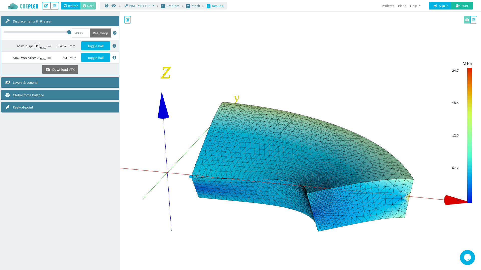
1.2.1 NAFEMS LE10 benchmark
Let us solve the linear elasticity benchmark problem NAFEMS LE10 “Thick plate pressure.” with FeenoX. Note the one-to-one correspondence between the human-friendly problem statement from fig. 3 and the FeenoX input file:

# NAFEMS Benchmark LE-10: thick plate pressure
PROBLEM mechanical MESH nafems-le10.msh   # mesh in millimeters

# LOADING: uniform normal pressure on the upper surface
BC upper    p=1      # 1 Mpa

# BOUNDARY CONDITIONS:
BC DCD'C'   v=0      # Face DCD'C' zero y-displacement
BC ABA'B'   u=0      # Face ABA'B' zero x-displacement
BC BCB'C'   u=0 v=0  # Face BCB'C' x and y displ. fixed
BC midplane w=0      #  z displacements fixed along mid-plane

# MATERIAL PROPERTIES: isotropic single-material properties
E = 210 * 1e3   # Young modulus in MPa
nu = 0.3        # Poisson's ratio

# print the direct stress y at D (and nothing more)
PRINTF "σ_y @ D = %.4f MPa" sigmay(2000,0,300)
Here, “one-to-one” means that the input file does not need any extra definition which is not part of the problem formulation. Of course the cognizant engineer can give further definitions such as
- the linear solver and pre-conditioner
- the tolerances for iterative solvers
- options for computing stresses out of displacements
- etc.
However, she is not obliged to as–at least for simple problems—the defaults are reasonable. This is akin to writing a text in Markdown where one does not need to care if the page is A4 or letter (as, in most cases, the output will not be printed but rendered in a web browser).
The problem asks for the normal stress in the y direction \sigma_y at point “D,” which is what FeenoX writes (and nothing else, rule of economy):
$ feenox nafems-le10.fee
sigma_y @ D =   -5.38016        MPa
$
Also note that since there is only one material, there is no need to do an explicit link between material properties and physical volumes in the mesh (rule of simplicity). And since the properties are uniform and isotropic, a single global scalar for E and a global single scalar for \nu are enough.
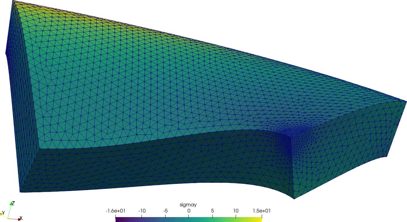
For the sake of visual completeness, post-processing data with the scalar distribution of \sigma_y and the vector field of displacements [u,v,w] can be created by adding one line to the input file:
WRITE_MESH nafems-le10.vtk sigmay VECTOR u v wThis VTK file can then be post-processed to create interactive 3D views, still screenshots, browser and mobile-friendly webGL models, etc. In particular, using Paraview one can get a colorful bitmapped PNG (the displacements are far more interesting than the stresses in this problem).
1.2.2 The Lorenz chaotic system
Let us consider the famous chaotic Lorenz’s dynamical system. Here is one way of getting an image of the butterfly-shaped attractor using FeenoX to compute it and Gnuplot to draw it. Solve
\begin{cases} \dot{x} &= \sigma \cdot (y - x) \\ \dot{y} &= x \cdot (r - z) - y \\ \dot{z} &= x y - b z \\ \end{cases}
for 0 < t < 40 with initial conditions
\begin{cases} x(0) = -11 \\ y(0) = -16 \\ z(0) = 22.5 \\ \end{cases}
and \sigma=10, r=28 and b=8/3, which are the classical parameters that generate the butterfly as presented by Edward Lorenz back in his seminal 1963 paper Deterministic non-periodic flow.
The following ASCII input file resembles the parameters, initial conditions and differential equations of the problem as naturally as possible:
PHASE_SPACE x y z     # Lorenz attractor’s phase space is x-y-z
end_time = 40         # we go from t=0 to 40 non-dimensional units

sigma = 10            # the original parameters from the 1963 paper
r = 28
b = 8/3

x_0 = -11             # initial conditions
y_0 = -16
z_0 = 22.5

# the dynamical system's equations written as naturally as possible
x_dot = sigma*(y - x)
y_dot = x*(r - z) - y
z_dot = x*y - b*z

PRINT t x y z        # four-column plain-ASCII output
Indeed, when executing FeenoX with this input file, we get four ASCII columns (t, x, y and z) which we can then redirect to a file and plot it with a standard tool such as Gnuplot. Note the importance of relying on plain ASCII text formats both for input and output, as recommended by the Unix philosophy and the rule of composition: other programs can easily create inputs for FeenoX and other programs can easily understand FeenoX’s outputs. This is essentially how Unix filters and pipes work.
Note the one-to-one correspondence between the human-friendly differential equations (written in TeX and rendered as typesetted mathematical symbols) and the computer-friendly input file that FeenoX reads.
Even though the initial version of FeenoX does not provide an API for high-level interpreted languages such as Python or Julia, the code is written in such a way that this feature can be added without needing a major refactoring. This will allow to fully define a problem in a procedural way, increasing also flexibility.
2 Architecture
The tool must be aimed at being executed unattended on remote servers which are expected to have a mainstream (as of the 2020s) architecture regarding operating system (GNU/Linux variants and other Unix-like OSes) and hardware stack, such as
- a few Intel-compatible or ARM-like CPUs per host
- a few levels of memory caches
- a few gigabytes of random-access memory
- several gigabytes of solid-state storage
It should successfully run on
- bare-metal
- virtual servers
- containerized images
using standard compilers, dependencies and libraries already available in the repositories of most current operating systems distributions.
Preference should be given to open source compilers, dependencies and libraries. Small problems might be executed in a single host but large problems ought to be split through several server instances depending on the processing and memory requirements. The computational implementation should adhere to open and well-established parallelization standards.
Ability to run on local desktop personal computers and/laptops is not required but suggested as a mean of giving the opportunity to users to test and debug small coarse computational models before launching the large computation on a HPC cluster or on a set of scalable cloud instances. Support for non-GNU/Linux operating systems is not required but also suggested.
Mobile platforms such as tablets and phones are not suitable to run engineering simulations due to their lack of proper electronic cooling mechanisms. They are suggested to be used to control one (or more) instances of the tool running on the cloud, and even to pre and post process results through mobile and/or web interfaces.
Very much like the C language (after A & B) and Unix itself (after a first attempt and the failed MULTICS), FeenoX can be seen as a third-system effect:
A notorious ‘second-system effect’ often afflicts the successors of small experimental prototypes. The urge to add everything that was left out the first time around all too frequently leads to huge and overcomplicated design. Less well known, because less common, is the ‘third-system effect’: sometimes, after the second system has collapsed of its own weight, there is a chance to go back to simplicity and get it right.
Feenox is indeed the third version written from scratch after a first implementation in 2009 (different small components with different names) and a second one (named wasora that allowed dynamically-shared plugins to be linked at runtime to provide particular PDEs) which was far more complex and had far more features circa 2012–2015. The third attempt, FeenoX, explicitly addresses the “do one thing well” idea from Unix.
Furthermore, not only is FeenoX itself both free and open-source software but, following the rule of composition (sec. 11.3), it also is designed to connect and to work with other free and open source software such as
- Gmsh for pre and/or post-processing
- ParaView for post-processing
- Gnuplot for plotting 1D/2D results
- Pyxplot for plotting 1D results
- Pandoc for creating tables and documents
- TeX for creating tables and documents
and many others, which are readily available in all major GNU/Linux distributions.
FeenoX also makes use of high-quality free and open source mathematical libraries which contain numerical methods designed by mathematicians and implemented by professional programmers. In particular, it depends on
- GNU Scientific Library for general mathematics,
- SUNDIALS IDA for ODEs and DAEs,
- PETSc for linear, non-linear and transient PDEs, and
- SLEPc for PDEs involving eigen problems
Therefore, if one zooms in into the block of the transfer function above, FeenoX can also be seen as a glue layer between the input files defining a physical problem and the mathematical libraries used to solve the discretized equations. For example, when solving the linear elastic problem from the NAFEMS LE10 case discussed above, we can draw the following diagram:
![]()
This way, FeenoX bounds its scope to do only one thing and to do it well: to build and solve finite-element formulations of physical problems. And it does so on high grounds, both ethical and technological:
Ethical, since it is free software, all users can
- run,
- share,
- modify, and/or
- re-share their modifications.
If a user cannot read or write code to make FeenoX suit her needs, at least she has the freedom to hire someone to do it for her.
Technological, since it is open source, advanced users can detect and correct bugs and even improve the algorithms. Given enough eyeballs, all bugs are shallow.
FeenoX’s main development architecture is Debian GNU/Linux running over 64-bits Intel-compatible processors (but binaries for ARM architectures can be compiled as well). All the dependencies are free and/or open source and already available in Debian’s latest stable official repositories, as explained in sec. 2.1.
The POSIX standard is followed whenever possible, allowing thus
FeenoX to be compiled in other operating systems and architectures such
as Windows (using Cygwin) and
MacOS. The build procedure is the well-known and mature
./configure && make command.
FeenoX is written in C conforming to the ISO C99 specification (plus POSIX extensions), which is a standard, mature and widely supported language with compilers for a wide variety of architectures. As listed above, for its basic mathematical capabilities, FeenoX uses the GNU Scientific Library. For solving ODEs/DAEs, FeenoX relies on Lawrence Livermore’s SUNDIALS library. For PDEs, FeenoX uses Argonne’s PETSc library and Universitat Politècnica de València’s SLEPc library. All of them are
- free and open source,
- written in C (neither Fortran nor C++),
- mature and stable,
- actively developed and updated,
- very well known both in the industry and academia.
Moreover, PETSc and SLEPc are scalable through the MPI standard, further discussed in sec. 2.4. This means that programs using both these libraries can run on either large high-performance supercomputers or low-end laptops. FeenoX has been run on
- Raspberry Pi
- Laptop (GNU/Linux & Windows 10)
- Macbook
- Desktop PC
- Bare-metal servers
- Vagrant/Virtualbox virtual machines
- Docker/Kubernetes containers
- AWS/DigitalOcean/Contabo instances
Due to the way that FeenoX is designed and the policy separated from the mechanism, it is possible to control a running instance remotely from a separate client which can eventually run on a mobile device (fig. 2,fig. 5).
The following example illustrates how well FeenoX works as one of many links in a chain that goes from tracing a bitmap with the problem’s geometry down to creating a nice figure with the results of a computation.

Say you are Homer J. Simpson and you want to solve a maze drawn in a restaurant’s placemat while driving to your wife’s aunt funeral. One where both the start and end points are known beforehand as show in fig. 7. In order to avoid falling into the alligator’s mouth, you can exploit the ellipticity of the Laplacian operator to solve any maze (even a hand-drawn one) without needing any fancy AI or ML algorithm. Just FeenoX and a bunch of standard open source tools to convert a bitmapped picture of the maze into an unstructured mesh.
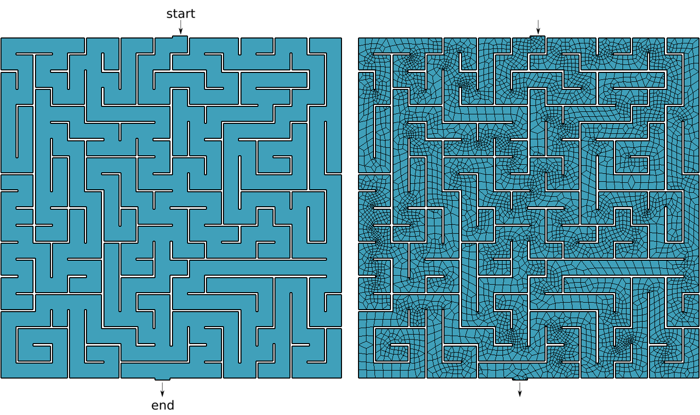
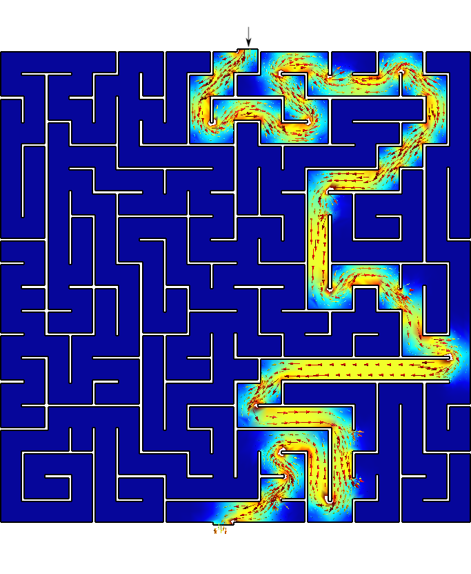
Figure 8: Bitmapped, meshed and solved mazes.. a — Bitmapped maze from https://www.mazegenerator.net (left) and 2D mesh (right), b — Solution to found by FeenoX (and drawn by Gmsh)
Create a maze
Download it in PNG (fig. 8 (a))
Perform some conversions
- PNG \rightarrow PNM \rightarrow SVG \rightarrow DXF \rightarrow GEO
$ wget http://www.mazegenerator.net/static/orthogonal_maze_with_20_by_20_cells.png
$ convert orthogonal_maze_with_20_by_20_cells.png -negate maze.png
$ potrace maze.pnm --alphamax 0  --opttolerance 0 -b svg -o maze.svg
$ ./svg2dxf maze.svg maze.dxf
$ ./dxf2geo maze.dxf 0.1
Open it with Gmsh
- Add a surface
- Set physical curves for “start” and “end”
Mesh it (fig. 8 (a))
gmsh -2 maze.geoSolve \nabla^2 \phi = 0 with BCs
\begin{cases} \phi=0 & \text{at “start”} \\ \phi=1 & \text{at “end”} \\ \nabla \phi \cdot \hat{\vec{n}} = 0 & \text{everywhere else} \\ \end{cases}
PROBLEM laplace 2D  # pretty self-descriptive, isn't it?
READ_MESH maze.msh

# boundary conditions (default is homogeneous Neumann)
BC start  phi=0
BC end    phi=1

SOLVE_PROBLEM

# write the norm of gradient as a scalar field
# and the gradient as a 2d vector into a .msh file
WRITE_MESH maze-solved.msh \
    sqrt(dphidx(x,y)^2+dphidy(x,y)^2) \
    VECTOR dphidx dphidy 0
$ feenox maze.fee $Open
maze-solved.msh, go to start and follow the gradient \nabla \phi!
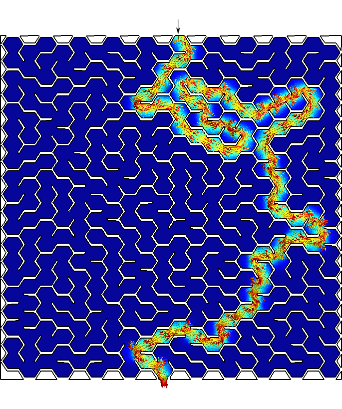
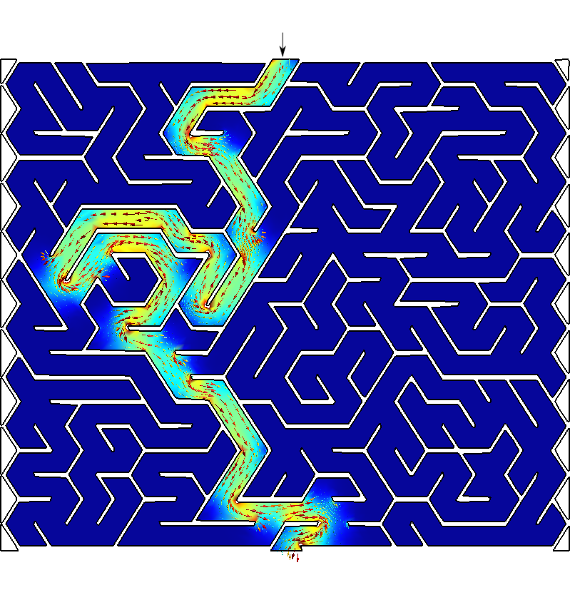
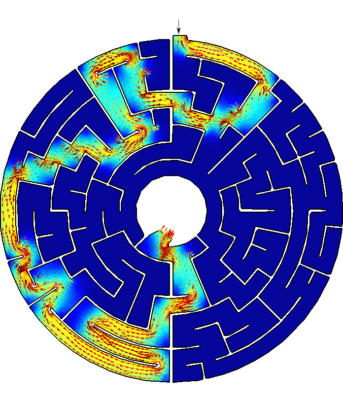
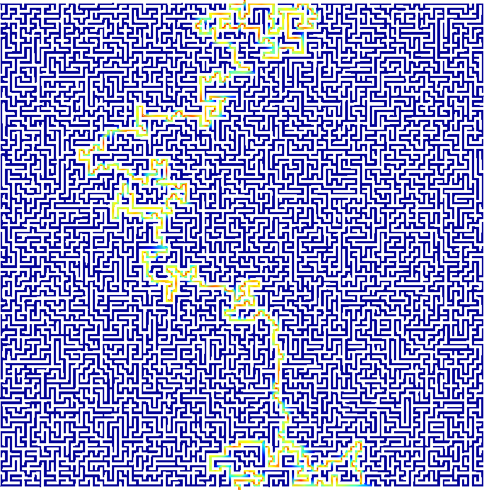
Figure 9: Any arbitrary maze (even hand-drawn) can be solved with FeenoX.
2.1 Deployment
The tool should be easily deployed to production servers. Both
- an automated method for compiling the sources from scratch aiming at obtaining optimized binaries for a particular host architecture should be provided using a well-established procedures, and
- one (or more) generic binary version aiming at common server architectures should be provided.
Either option should be available to be downloaded from suitable online sources, either by real people and/or automated deployment scripts.
As already stated, FeenoX can be compiled from its sources using the
well-established configure & make
procedure. The code’s source tree is hosted on Github so cloning the
repository is the preferred way to obtain FeenoX, but source tarballs
are periodically released too according to the requirements in sec. 4.1.
There are also non-official binary .deb packages which can
be installed with apt using a custom package repository
location.
The configuration and compilation is based on GNU Autotools that has more than thirty years of maturity and it is the most portable way of compiling C code in a wide variety of Unix variants. It has been tested with
- GNU C compiler (free)
- LLVM Clang compiler (free)
- Intel oneAPI C compiler (privative)
FeenoX depends on the four open source libraries stated in sec. 2,
although the last three of them are optional. The only mandatory library
is the GNU Scientific Library which is part of the GNU/Linux operating
system and as such is readily available in all distributions as
libgsl-dev. The sources of the rest of the optional
libraries are also widely available in most common GNU/Linux
distributions.
In effect, doing
sudo apt-get install gcc make libgsl-dev libsundials-dev petsc-dev slepc-devis enough to provision all the dependencies needed compile FeenoX from the source tarball with the full set of features. If using the Git repository as a source, then Git itself and the GNU Autoconf and Automake packages are also needed:
sudo apt-get install git autoconf automakeEven though compiling FeenoX from sources is the recommended way to
obtain the tool—since the target binary can be compiled using
particularly suited compilation options, flags and optimizations
(especially those related to MPI, linear algebra kernels and direct
and/or iterative sparse solvers)–there are also tarballs and
.deb packages with usable binaries for some of the most
common architectures—including some non-GNU/Linux variants. These binary
distributions contain statically-linked executable files that do not
need any other shared libraries to be installed on the target host.
However, their flexibility and efficiency is generic and far from ideal.
Yet the flexibility of having an execution-ready distribution package
for users that do not know how to compile C source code outweighs the
limited functionality and scalability of the tool.
For example, first PETSc can be built with a -Ofast
flag:
$ cd $PETSC_DIR
$ export PETSC_ARCH=linux-fast
$ ./configure --with-debug=0 COPTFLAGS="-Ofast"
$ make -j8
$ cd $HOMEAnd then not only can FeenoX be configured to use that particular
PETSc build but also to use a different compiler such as Clang instead
of GNU GCC and to use the same -Ofast flag to compile
FeenoX itself:
$ git clone https://github.com/seamplex/feenox
$ cd feenox
$ ./autogen.sh
$ export PETSC_ARCH=linux-fast
$ ./configure MPICH_CC=clang CFLAGS=-Ofast
$ make -j8
# make installIf one does not care about the details of the compilation, then a pre-compiled statically-linked binary can be directly downloaded very much as when downloading Gmsh:
$ wget http://gmsh.info/bin/Linux/gmsh-Linux64.tgz
$ wget https://seamplex.com/feenox/dist/linux/feenox-linux-amd64.tar.gzAppendix sec. 13 has more details about how to download and compile FeenoX. The full online documentation contains a compilation guide with further detailed explanations of each of the steps involved.
All the commands needed to either download a binary executable or to
compile from source with customized optimization flags can be automated.
The repository contains a subdirectory dist
with instructions and scripts to build
- source tarballs
- binary tarballs
- Debian-compatible
.debpackages
This way, deployment of the solver can be customized and tweaked as needed, including creating Docker containers with a working version of FeenoX.
2.2 Execution
It is mandatory to be able to execute the tool remotely, either with a direct action from the user or from a high-level workflow which could be triggered by a human or by an automated script. Since it is required for the tool to be able to be run distributed among different servers, proper means to perform this kind of remote executions should be provided. The calling party should be able to monitor the status during run time and get the returned error level after finishing the execution.
The tool shall provide means to perform parametric computations by varying one or more problem parameters in a certain prescribed way such that it can be used as an inner solver for an outer-loop optimization tool. In this regard, it is desirable that the tool could compute scalar values such that the figure of merit being optimized (maximum temperature, total weight, total heat flux, minimum natural frequency, maximum displacement, maximum von Mises stress, etc.) is already available without needing further post-processing.
As requested by the SRS and explained in sec. 1.2, FeenoX is a program that reads the problem to be solved at run-time and not a library that has to be linked against code that defines the problem. Since FeenoX is designed to run as
- a Unix filter, or
- as a transfer function between input and output files
and it explicitly avoids having a graphical interface, the binary
executable works as any other Unix terminal command. Moreover, as
discussed in sec. 2.4, FeenoX uses the MPI standard for parallelization
among several hosts. Therefore, it can be launched through the command
mpiexec
(or
mpirun).
When invoked without arguments, it prints its version (a thorough explanation of the versioning scheme is given in sec. 4.1), a one-line description and the usage options:
$ feenox
FeenoX v1.0.8-g731ca5d
a cloud-first free no-fee no-X uniX-like finite-element(ish) computational engineering tool
usage: feenox [options] inputfile [replacement arguments] [petsc options]
-h, --help display options and detailed explanations of command-line usage
-v, --version display brief version information and exit
-V, --versions display detailed version information
-c, --check validates if the input file is sane or not
--pdes list the types of PROBLEMs that FeenoX can solve, one per line
--elements_info output a document with information about the supported element types
--linear force FeenoX to solve the PDE problem as linear
--non-linear force FeenoX to solve the PDE problem as non-linear
Run with --help for further explanations.
$The program can also be executed remotely either
- on a running server through a SSH session
in serial directly invoking the
feenoxbinaryin parallel through the
mpiexecwrapper, e.g.mpiexec -n 4 feenox input.fee
- spawned by a daemon listening to a network requests,
- in a container as part of a provisioning script,
- in many other ways.
As explained in the help message, FeenoX can read the input from the
standard input if - is specified as the input path. This is
useful in scripts where small calculations are needed, e.g.
$ a=3
$ echo "PRINT 1/$a" | feenox -
0.333333
$ FeenoX provides mechanisms to inform its progress by writing certain
information to devices or files, which in turn can be monitored remotely
or even trigger server actions. Progress can be as simple as an ASCII
bar (triggered with --progress in the command line or with
the keyword PROGRESS
in the input file) to more complex mechanisms like writing the status in
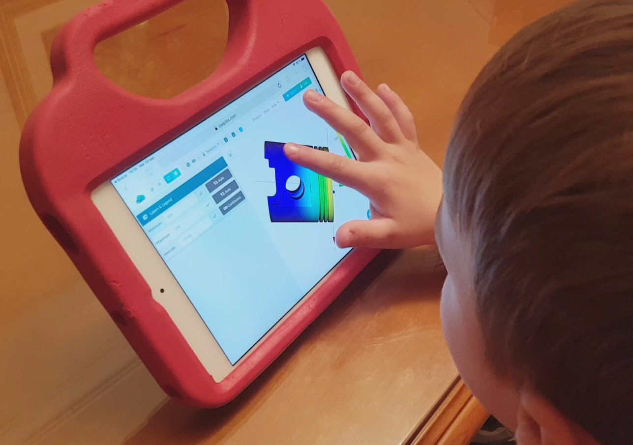
a shared memory segment. Fig. 10 shows how the CAEplex platform shows the progress
interactively in its web-based interface.
Regarding its execution, there are three ways of solving problems:
- direct execution
- parametric runs, and
- optimization loops.
2.2.1 Direct execution
When directly executing FeenoX, one gives a single argument to the executable with the path to the main input file. For example, the following input computes the first twenty numbers of the Fibonacci sequence using the closed-form formula
f(n) = \frac{\varphi^n - (1-\varphi)^n}{\sqrt{5}}
where \varphi=(1+\sqrt{5})/2 is the Golden ratio:
# the Fibonacci sequence using the closed-form formula as a function
phi = (1+sqrt(5))/2
f(n) = (phi^n - (1-phi)^n)/sqrt(5)
PRINT_FUNCTION f MIN 1 MAX 20 STEP 1FeenoX can be directly executed to print the function f(n) for n=1,\dots,20 both to the standard output and
to a file named one (because it is the first way of solving
Fibonacci with Feenox):
$ feenox fibo_formula.fee | tee one
1 1
2 1
3 2
4 3
5 5
6 8
7 13
8 21
9 34
10 55
11 89
12 144
13 233
14 377
15 610
16 987
17 1597
18 2584
19 4181
20 6765
$Now, we could also have computed these twenty numbers by using the
direct definition of the sequence into a vector \vec{f} of size 20. This time we redirect the
output to a file named two:
# the fibonacci sequence as a vector
VECTOR f SIZE 20
f[i]<1:2> = 1
f[i]<3:vecsize(f)> = f[i-2] + f[i-1]
PRINT_VECTOR i f$ feenox fibo_vector.fee > two
$ Finally, we print the sequence as an iterative problem and check that the three outputs are the same:
# the fibonacci sequence as an iterative problem
static_steps = 20
#static_iterations = 1476 # limit of doubles
IF step_static=1|step_static=2
f_n = 1
f_nminus1 = 1
f_nminus2 = 1
ELSE
f_n = f_nminus1 + f_nminus2
f_nminus2 = f_nminus1
f_nminus1 = f_n
ENDIF
PRINT step_static f_n$ feenox fibo_iterative.fee > three
$ diff one two
$ diff two three
$These three calls were examples of direct execution of FeenoX: a single call with a single argument to solve a single fixed problem.
2.2.2 Parametric
To use FeenoX in a parametric run, one has to successively call the
executable passing the main input file path in the first argument
followed by an arbitrary number of parameters. These extra parameters
will be expanded as string literals $1, $2,
etc. appearing in the input file. For example, if hello.fee
is
PRINT "Hello $1!"then
$ feenox hello.fee World
Hello World!
$ feenox hello.fee Universe
Hello Universe!
$To have an actual parametric run, an external loop has to
successively call FeenoX with the parametric arguments. For example, say
this file cantilever.fee fixes the face called “left” and
sets a load in the negative z direction
of a mesh called cantilever-$1-$2.msh. The output is a
single line containing the number of nodes of the mesh and the
displacement in the vertical direction w(500,0,0) at the center of the cantilever’s
free face:
PROBLEM elastic 3D
READ_MESH cantilever-$1-$2.msh # in meters
E = 2.1e11 # Young modulus in Pascals
nu = 0.3 # Poisson's ratio
BC left fixed
BC right tz=-1e5 # traction in Pascals, negative z
SOLVE_PROBLEM
# z-displacement (components are u,v,w) at the tip vs. number of nodes
PRINT nodes w(500,0,0) "\# $1 $2"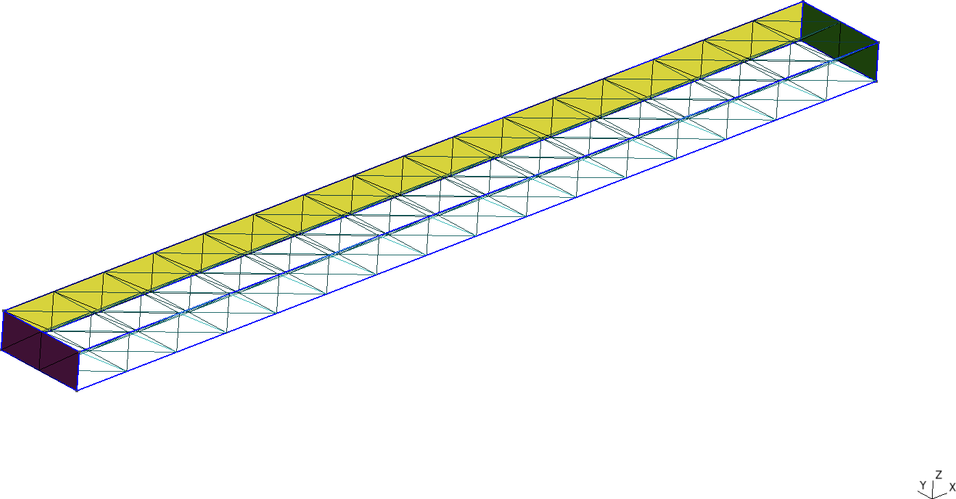
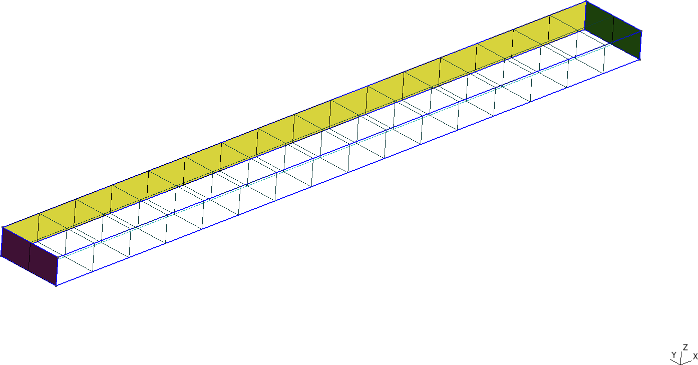
Figure 11: Cantilevered beam meshed with structured tetrahedra and hexahedra. a — Tetrahedra, b — Hexahedra
Now the following Bash script
first calls Gmsh to create the meshes
cantilever-${element}-${c}.msh where
${element}: tet4, tet10, hex8, hex20, hex27${c}: 1,2,,10
It then calls FeenoX with the input above and passes
${element} and ${c} as extra arguments, which
then are expanded as $1 and $2
respectively.
#!/bin/bash
rm -f *.dat
for element in tet4 tet10 hex8 hex20 hex27; do
for c in $(seq 1 10); do
# create mesh if not already cached
mesh=cantilever-${element}-${c}
if [ ! -e ${mesh}.msh ]; then
scale=$(echo "PRINT 1/${c}" | feenox -)
gmsh -3 -v 0 cantilever-${element}.geo -clscale ${scale} -o ${mesh}.msh
fi
# call FeenoX
feenox cantilever.fee ${element} ${c} | tee -a cantilever-${element}.dat
done
doneAfter the execution of the script, thanks to the design decision
(explained in sec. 3.2) that output is 100% defined by the user (in this
case with the PRINT
instruction), one has several files
cantilever-${element}.dat files. When plotted, these show
the shear locking effect of fully-integrated first-order elements as
illustrated in fig. 12. The theoretical Euler-Bernoulli
result is just a reference as, among other things, it does not take into
account the effect of the material’s Poisson’s
ratio. Note that the abscissa shows the number of nodes,
which are proportional to the number of degrees of freedom (i.e. the
size of the problem matrix) and not the number of elements,
which is irrelevant here and in most problems.

2.2.3 Optimization loops
Optimization loops work very much like parametric runs from the FeenoX point of view. The difference is mainly on the calling script that has to implement a certain optimization algorithm such as conjugate gradients, Nelder-Mead, simulated annealing, genetic algorithms, etc. to choose which parameters to pass to FeenoX as command-line argument. The only particularity on FeenoX’s side is that since the next argument that the optimization loop will pass might depend on the result of the current step, care has to be taken in order to be able to return back to the calling script whatever results it needs in order to compute the next arguments. This is usually just the scalar being optimized for, but it can also include other results such as derivatives or other relevant data.
To illustrate how to use FeenoX in an optimization loop, let us consider the problem of finding the length \ell_1 of a tuning fork (fig. 13) such that the fundamental frequency on a free-free oscillation is equal to the base A frequency at 440 Hz.

This extremely simple input file (rule of simplicity sec. 11.5) solves the free-free mechanical modal problem (i.e. without any Dirichlet boundary condition) and prints the fundamental frequency:
PROBLEM modal 3D MODES 1 # only one mode needed
READ_MESH fork.msh # in [m]
E = 2.07e11 # in [Pa]
nu = 0.33
rho = 7829 # in [kg/m^2]
# no BCs! It is a free-free vibration problem
SOLVE_PROBLEM
# write back the fundamental frequency to stdout
PRINT f(1)Note that in this particular case, the FeenoX input files does not
expand any command-line argument. The trick is that the mesh file
fork.msh is overwritten in each call of the optimization
loop. Since this time the loop is slightly more complex than in the
parametric run of the last section, we now use Python. The function
create_mesh() first creates a CAD model of the fork with
geometrical parameters r, w, \ell_1
and \ell_2. It then meshes the CAD
using n structured hexahedra through
the fork’s thickness. Both the CAD and the mesh are created using the
Gmsh Python API. The detailed steps between
gmsh.initialize() and gmsh.finalize() are not
shown here, just the fact that this function overwrites the previous
mesh and always writes it into the file called fork.msh
which is the one that fork.fee reads. Hence, there is no
need to pass command-liner arguments to FeenoX. The full implementation
of the function is available in the examples directory of the FeenoX
distribution.
import math
import gmsh
import subprocess # to call FeenoX and read back
def create_mesh(r, w, l1, l2, n):
gmsh.initialize()
...
gmsh.write("fork.msh")
gmsh.finalize()
return len(nodes)
def main():
target = 440 # target frequency
eps = 1e-2 # tolerance
r = 4.2e-3 # geometric parameters
w = 3e-3
l1 = 30e-3
l2 = 60e-3
for n in range(1,7): # mesh refinement level
l1 = 60e-3 # restart l1 & error
error = 60
while abs(error) > eps: # loop
l1 = l1 - 1e-4*error
# mesh with Gmsh Python API
nodes = create_mesh(r, w, l1, l2, n)
# call FeenoX and read scalar back
# TODO: FeenoX Python API (like Gmsh)
result = subprocess.run(['feenox', 'fork.fee'], stdout=subprocess.PIPE)
freq = float(result.stdout.decode('utf-8'))
error = target - freq
print(nodes, l1, freq)Since the computed frequency depends both on the length \ell_1 and on the mesh refinement level n, there are actually two nested loops: one parametric over n=1,2\dots,7 and the optimization loop itself that tries to find \ell_1 so as to obtain a frequency equal to 440 Hz within 0.01% of error.
$ python fork.py > fork.dat
$
Note that the approach used here is to use Gmsh Python API to build
the mesh and then fork the FeenoX executable to solve the fork (no pun
intended). There are plans to provide a Python API for FeenoX so the
problem can be set up, solved and the results read back directly from
the script instead of needing to do a fork+exec, read back the standard
output as a string and then convert it to a Python
float.
Fig. 14 shows the results of the combination of the optimization loop over \ell_1 and a parametric run over n. The difference for n=6 and n=7 is in the order of one hundredth of millimeter.
2.3 Efficiency
As required in the previous section, it is mandatory to be able to execute the tool on one or more remote servers. The computational resources needed from this server, i.e. costs measured in
- CPU/GPU time
- random-access memory
- long-term storage
- etc.
needed to solve a problem should be comparable to other similar state-of-the-art cloud-based script-friendly finite-element tools.
One of the most widely known quotations in computer science is that one that says “premature optimization is the root of all evil.” that is an extremely over-simplified version of Donald E. Knuth’s analysis in his The Art of Computer Programming. Bottom line is that the programmer should not not spend too much time trying to optimize code based on hunches but based on profiling measurements. Yet a disciplined programmer can tell when an algorithm will be way too inefficient (say something that scales up like O(n^2)) and how small changes can improve performance (say by understanding how caching levels work in order to implement faster nested loops). It is also true that usually an improvement in one aspect leads to a deterioration in another one (e.g. a decrease in CPU time by caching intermediate results in an increase of RAM usage).
Even though FeenoX is still evolving so it could be premature in many cases, it is informative to compare running times and memory consumption when solving the same problem with different cloud-friendly FEA programs. In effect, a serial single-thread single-host comparison of resource usage when solving the NAFEMS LE10 problem introduced above was performed, using both unstructured tetrahedral and structured hexahedral meshes. Fig. 15 shows two figures of the many ones contained in the detailed report. In general, FeenoX using the iterative approach based on PETSc’s Geometric-Algebraic Multigrid Preconditioner and a conjugate gradients solver is faster for (relatively) large problems at the expense of a larger memory consumption. The curves that use MUMPS confirm the well-known theoretical result that direct linear solvers are robust but not scalable.


Figure 15: Resource consumption when solving the NAFEMS LE10 problem in the cloud for tetrahedral meshes.. a — Wall time vs. number of degrees of freedom, b — Memory vs. number of degrees of freedom
Regarding storage, FeenoX needs space to store the input file
(negligible), the mesh file in .msh format (which can be
either ASCII or binary) and the optional output files in
.msh or .vtu/.vtk formats. All of
these files can be stored gzip-compressed and un-compressed on demand by
exploiting FeenoX’s script-friendliness using proper calls to
gzip before and/or after calling the feenox
binary.
2.4 Scalability
The tool ought to be able to start solving small problems first to check the inputs and outputs behave as expected and then allow increasing the problem size up in order to achieve to the desired accuracy of the results. As mentioned in sec. 2, large problem should be split among different computers to be able to solve them using a finite amount of per-host computational power (RAM and CPU).
When for a fixed problem the mesh is refined over and over, more and more computational resources are needed to solve it (and to obtain more accurate results, of course). Parallelization can help to
- reduce the wall time needed to solve a problem by using several processors at the same time
- allow to solve big problems that would not fit into a single computer by splitting them into smaller parts, each of them fitting in a single computer
There are three types of parallelization schemes:
- Shared-memory systems (OpenMP)
-
several processing units sharing a single memory address space
- Distributed systems (MPI)
-
several computational units, each with their own processing units and memory, inter-connected with high-speed network hardware
- Graphical processing units (GPU)
-
used as co-processors to solve numerically-intensive problems
In principle, any of these three schemes can be used to reduce the wall time (a). But only the distributed systems scheme allows to solve arbitrarily big problems (b).
It might seem that the most effective approach to solve a large problem is to use OpenMP (not to be confused with OpenMPI!) among threads running in processors that share the memory address space and to use MPI among processes running in different hosts. But even though this hybrid OpenMP+MPI scheme is possible, there are at least three main drawbacks with respect to a pure MPI approach:
- the overall performance is not be significantly better
- the amount of lines of code that has to be maintained is more than doubled
- the number of possible points of synchronization failure increases
In many ways, the pure MPI mode has fewer synchronizations and thus should perform better. Hence, FeenoX uses MPI (mainly through PETSc and SLEPc) to handle large parallel problems.
To illustrate FeenoX’s MPI features, let us consider the following input file (which is part of FeenoX’s tests suite):
PRINTF_ALL "Hello MPI World!"The instruction PRINTF_ALL (at the end of the day, it is
a verb) asks all the processes to write the
printf-formatted arguments in the standard output. A prefix
is added to each line with the process id and the name of the host. When
running FeenoX with this input file through mpiexec in an
AWS server which has already been properly configured to connect to
another one and split the MPI processes, we get:
ubuntu@ip-172-31-44-208:~/mpi/hello$ mpiexec --verbose --oversubscribe --hostfile hosts -np 4 ./feenox hello_mpi.fee
[0/4 ip-172-31-44-208] Hello MPI World!
[1/4 ip-172-31-44-208] Hello MPI World!
[2/4 ip-172-31-34-195] Hello MPI World!
[3/4 ip-172-31-34-195] Hello MPI World!
ubuntu@ip-172-31-44-208:~/mpi/hello$ That is to say,host ip-172-31-44-208 spawns two local
processes feenox and, at the same time, asks host
ip-172-31-34-195 to create two new processes in it. This
scheme would allow to solve a problem in parallel where the CPU and RAM
loads are split into two different servers.

We can used Gmsh’s tutorial t21 that illustrated the
concept of domain decomposition (DDM) to show another aspect of how MPI
parallelization works in FeenoX. In effect, let us consider the mesh
from fig. 16 that consists of two non-dimensional squares of size 1 \times 1 and let us say we want to compute
the integral of the constant 1 over the surface to obtain the numerical
result 2.
READ_MESH t21.msh
INTEGRATE 1 RESULT two
PRINTF_ALL "%g" twoIn this case, the instruction INTEGRATE is executed in
parallel where each process computes the local contribution and, before
moving into the next instruction (PRINTF_ALL), all
processes synchronize and sum up all these contributions (i.e. they
perform a sum reduction) and all the processes obtain the global result
in the variable two:
$ mpiexec -n 2 feenox t21.fee
[0/2 tom] 2
[1/2 tom] 2
$ mpiexec -n 4 feenox t21.fee
[0/4 tom] 2
[1/4 tom] 2
[2/4 tom] 2
[3/4 tom] 2
$ mpiexec -n 6 feenox t21.fee
[0/6 tom] 2
[1/6 tom] 2
[2/6 tom] 2
[3/6 tom] 2
[4/6 tom] 2
[5/6 tom] 2
$ To illustrate what is happening under the hood, let us temporarily modify the FeenoX source code so that each process shows the local contribution:
$ mpiexec -n 2 feenox t21.fee
[process 0] my local integral is 0.996699
[process 1] my local integral is 1.0033
[0/2 tom] 2
[1/2 tom] 2
$ mpiexec -n 3 feenox t21.fee
[process 0] my local integral is 0.658438
[process 1] my local integral is 0.672813
[process 2] my local integral is 0.668749
[0/3 tom] 2
[1/3 tom] 2
[2/3 tom] 2
$ mpiexec -n 4 feenox t21.fee
[process 0] my local integral is 0.505285
[process 1] my local integral is 0.496811
[process 2] my local integral is 0.500788
[process 3] my local integral is 0.497116
[0/4 tom] 2
[1/4 tom] 2
[2/4 tom] 2
[3/4 tom] 2
$ mpiexec -n 5 feenox t21.fee
[process 0] my local integral is 0.403677
[process 1] my local integral is 0.401883
[process 2] my local integral is 0.399116
[process 3] my local integral is 0.400042
[process 4] my local integral is 0.395281
[0/5 tom] 2
[1/5 tom] 2
[2/5 tom] 2
[3/5 tom] 2
[4/5 tom] 2
$ mpiexec -n 6 feenox t21.fee
[process 0] my local integral is 0.327539
[process 1] my local integral is 0.330899
[process 2] my local integral is 0.338261
[process 3] my local integral is 0.334552
[process 4] my local integral is 0.332716
[process 5] my local integral is 0.336033
[0/6 tom] 2
[1/6 tom] 2
[2/6 tom] 2
[3/6 tom] 2
[4/6 tom] 2
[5/6 tom] 2
$ Note that in the cases with 4 and 5 processes, the number of partitions P is not a multiple of the number of processes N. Anyway, FeenoX is able to distribute the load is able to distribute the load among the N processes, even though the efficiency is slightly less than in the other cases. :::
When solving PDEs, FeenoX builds the local matrices and vectors and then asks PETSc to assemble the global objects by sending non-local information as MPI messages. This way, all processes have contiguous rows as local data and the system of equations can be solved in parallel using the distributed system paradigm.
We can show that both
- the wall time, and
- the per-process memory
decrease when running a fixed-sized problem with MPI in parallel using the IAEA 3D PWR benchmark:
PROBLEM neutron_diffusion 3D GROUPS 2
DEFAULT_ARGUMENT_VALUE 1 quarter
READ_MESH iaea-3dpwr-$1.msh
MATERIAL fuel1 D1=1.5 D2=0.4 Sigma_s1.2=0.02 Sigma_a1=0.01 Sigma_a2=0.08 nuSigma_f2=0.135
MATERIAL fuel2 D1=1.5 D2=0.4 Sigma_s1.2=0.02 Sigma_a1=0.01 Sigma_a2=0.085 nuSigma_f2=0.135
MATERIAL fuel2rod D1=1.5 D2=0.4 Sigma_s1.2=0.02 Sigma_a1=0.01 Sigma_a2=0.13 nuSigma_f2=0.135
MATERIAL reflector D1=2.0 D2=0.3 Sigma_s1.2=0.04 Sigma_a1=0 Sigma_a2=0.01 nuSigma_f2=0
MATERIAL reflrod D1=2.0 D2=0.3 Sigma_s1.2=0.04 Sigma_a1=0 Sigma_a2=0.055 nuSigma_f2=0
BC vacuum vacuum=0.4692
BC mirror mirror
SOLVE_PROBLEM
WRITE_RESULTS FORMAT vtk
PRINT "geometry = $1"
PRINTF " keff = %.5f" keff
PRINTF " nodes = %g" nodes
PRINTF " DOFs = %g" total_dofs
PRINTF " memory = %.1f Gb (local) %.1f Gb (global)" mpi_memory_local() mpi_memory_global()
PRINTF " wall = %.1f sec" wall_time()$ mpiexec -n 1 feenox iaea-3dpwr.fee quarter
geometry = quarter
keff = 1.02918
nodes = 70779
DOFs = 141558
[0/1 tux] memory = 2.3 Gb (local) 2.3 Gb (global)
wall = 26.2 sec
$ mpiexec -n 2 feenox iaea-3dpwr.fee quarter
geometry = quarter
keff = 1.02918
nodes = 70779
DOFs = 141558
[0/2 tux] memory = 1.5 Gb (local) 3.0 Gb (global)
[1/2 tux] memory = 1.5 Gb (local) 3.0 Gb (global)
wall = 17.0 sec
$ mpiexec -n 4 feenox iaea-3dpwr.fee quarter
geometry = quarter
keff = 1.02918
nodes = 70779
DOFs = 141558
[0/4 tux] memory = 1.0 Gb (local) 3.9 Gb (global)
[1/4 tux] memory = 0.9 Gb (local) 3.9 Gb (global)
[2/4 tux] memory = 1.1 Gb (local) 3.9 Gb (global)
[3/4 tux] memory = 0.9 Gb (local) 3.9 Gb (global)
wall = 13.0 sec
$ 2.5 Flexibility
The tool should be able to handle engineering problems involving different materials with potential spatial and time-dependent properties, such as temperature-dependent thermal expansion coefficients and/or non-constant densities. Boundary conditions must be allowed to depend on both space and time as well, like non-uniform pressure loads and/or transient heat fluxes.
The third-system effect mentioned in sec. 2 involves more than ten
years of experience in the nuclear industry,4
where complex dependencies of multiple material properties over space
through intermediate distributions (temperature, neutronic poisons,
etc.) and time (control rod positions, fuel burn-up, etc.) are
mandatory. One of the cornerstone design decisions in FeenoX is that
everything is an expression (sec. 3.1.5). Here,
“everything” means any location in the input file where a numerical
value is expected. The most common use case is in the PRINT
keyword. For example, the Sophomore’s
dream (in contrast to Freshman’s
dream) identity
\int_{0}^{1} x^{-x} \, dx = \sum_{n=1}^{\infty} n^{-n}
can be illustrated like this:
VAR x
PRINT %.7f integral(x^(-x),x,0,1)
VAR n
PRINT %.7f sum(n^(-n),n,1,1000)$ feenox sophomore.fee
1.2912861
1.2912860
$Of course most engineering problems will not need explicit integrals—although a few of them do—but some might need summation loops, so it is handy to have these functionals available inside the FEA tool. This might seem to go against the “keep it simple” and “do one thing good” Unix principle, but definitely follows Alan Kay’s idea that “simple things should be simple, complex things should be possible” (further discussion in sec. 3.1.4).
Flexibility in defining non-trivial material properties is illustrated with the following example, where two squares made of different dimensionless materials are juxtaposed in thermal contact (glued?) and subject to different boundary conditions at each of the four sides (fig. 17).

The yellow square is made of a certain material with a conductivity that depends algebraically (and fictitiously) the temperature like
k_\text{yellow}(x,y) = \frac{1}{2} + T(x,y)
The cyan square has a space-dependent temperature given by a table of scattered data as a function of the spatial coordinates x and y (origin is left bottom corner of the yellow square) without any particular structure on the definition points:
| x | y | k_\text{cyan}(x,y) |
|---|---|---|
| 1 | 0 | 1.0 |
| 1 | 1 | 1.5 |
| 2 | 0 | 1.3 |
| 2 | 1 | 1.8 |
| 1.5 | 0.5 | 1.7 |
The cyan square generates a temperature-dependent power density (per unit area) given by
q^{\prime \prime}_\text{cyan}(x,y) = 0.2 \cdot T(x,y)
The yellow one does not generate any power so q^{\prime \prime}_\text{yellow} = 0. Boundary conditions are
\begin{cases} T(x,y) = y & \text{at the left edge $y=0$} \\ T(x,y) = 1-\cos\left(\frac{1}{2}\pi \cdot x\right) & \text{at the bottom edge $x=0$} \\ q'(x,y) = 2-y & \text{at the right edge $x=2$} \\ q'(x,y) = 1 & \text{at the top edge $y=1$} \\ \end{cases}
The input file illustrate how flexible FeenoX is and, again, how the problem definition in a format that the computer can understand resembles the humanly-written formulation of the original engineering problem:
PROBLEM thermal 2d # heat conduction in two dimensions
READ_MESH two-squares.msh
k_yellow(x,y) = 1/2+T(x,y) # thermal conductivity
FUNCTION k_cyan(x,y) INTERPOLATION shepard DATA {
1 0 1.0
1 1 1.5
2 0 1.3
2 1 1.8
1.5 0.5 1.7 }
q_cyan(x,y) = 1-0.2*T(x,y) # dissipated power density
q_yellow(x,y) = 0
BC left T=y # temperature (dirichlet) bc
BC bottom T=1-cos(pi/2*x)
BC right q=2-y # heat flux (neumann) bc
BC top q=1
SOLVE_PROBLEM
WRITE_MESH two-squares-results.msh T #CELLS kNote that FeenoX is flexible enough to…
- handle mixed meshes (the yellow square is meshed with triangles and the other one with quadrangles)
- use point-wise defined properties even though there is not
underlying structure nor topology for the points where the data is
defined (FeenoX could have read data from a
.mshor.vtkfile respecting the underlying topology) - understand that the problem is non-linear so as to use PETSc’s SNES framework automatically (the conductivity and power source depend on the temperature).
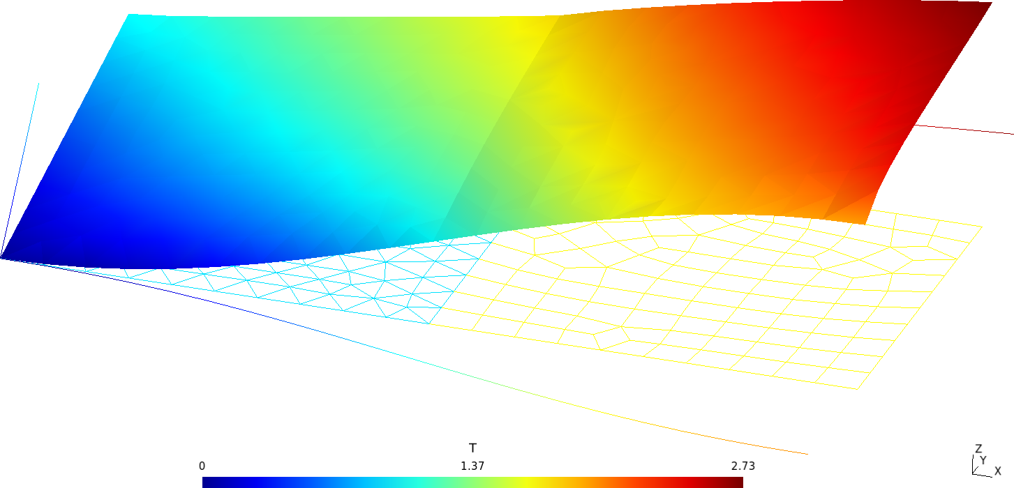
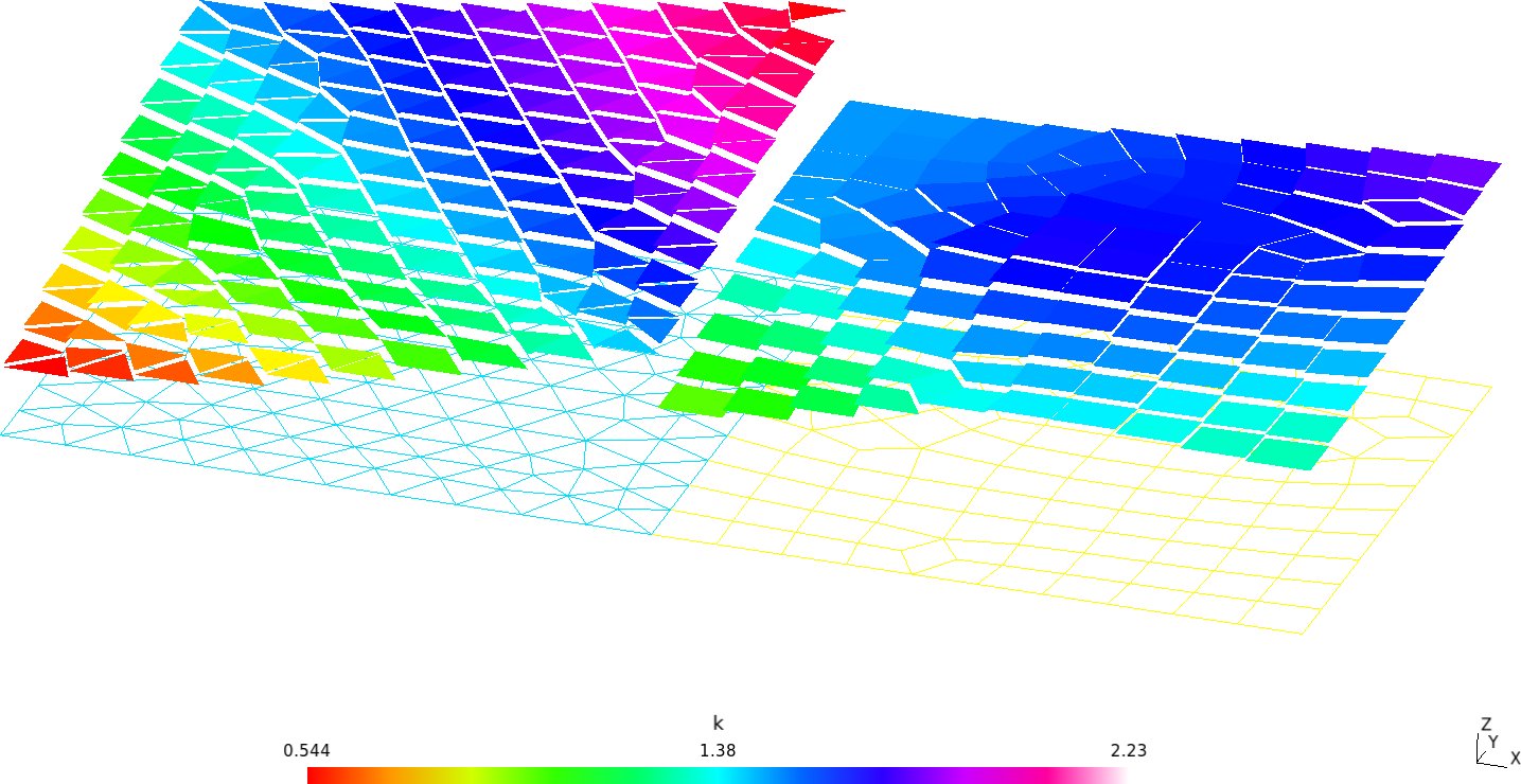
Figure 18: Temperature (main result) and conductivity for the two-squares thermal problem.. a — Temperature defined at nodes, b — Conductivity defined at cells
In the very same sense that variables x, y
and z appearing in the input refer to the spatial
coordinates x, y and z
respectively, the special variable t refers to the
time t. The requirement of allowing
time-dependent boundary conditions can be illustrated by solving the
NAFEMS T3 one-dimensional transient heat transfer benchmark. It consists
of a slab of 0.1 meters long subject to a fixed homogeneous temperature
on one side, i.e.
T(x=0)=0~\text{°C}
and to a transient temperature
T(x=0.1~\text{m},t)=100~\text{°C} \cdot \sin\left( \frac{\pi \cdot t}{40~\text{s}}\right)
at the other side. There is zero internal heat generation, at t=0 all temperature is equal to 0°C (sic) and conductivity, specific heat and density are constant and uniform. The problem asks for the temperature at location x=0.08~\text{m} at time t=32~\text{s}. The reference result is T(0.08~\text{m},32~\text{s})=36.60~\text{°C}.
PROBLEM thermal DIM 1 # NAFEMS-T3 benchmark: 1d transient heat conduction
READ_MESH slab-0.1m.msh
end_time = 32 # transient up to 32 seconds
T_0(x) = 0 # initial condition "all temperature is equal to 0°C"
# prescribed temperatures as boundary conditions
BC left T=0
BC right T=100*sin(pi*t/40)
# uniform and constant properties
k = 35.0 # conductivity [W/(m K)]
cp = 440.5 # heat capacity [J/(kg K)]
rho = 7200 # density [kg/m^3]
SOLVE_PROBLEM
# print detailed evolution into an ASCII file
PRINT FILE nafems-t3.dat %.3f t dt %.2f T(0.05) T(0.08) T(0.1)
# print the asked result into the standard output
IF done
PRINT "T(0.08m,32s) = " T(0.08) "ºC"
ENDIF$ gmsh -1 slab-0.1m.geo
[...]
Info : Done meshing 1D (Wall 0.000213023s, CPU 0.000836s)
Info : 61 nodes 62 elements
Info : Writing 'slab-0.1m.msh'...
Info : Done writing 'slab-0.1m.msh'
Info : Stopped on Sun Dec 12 19:41:18 2021 (From start: Wall 0.00293443s, CPU 0.02605s)
$ feenox nafems-t3.fee
T(0.08m,32s) = 36.5996 ºC
$ pyxplot nafems-t3.ppl
$
Besides “everything is an expression,” FeenoX follows another cornerstone rule: simple problems ought to have simple inputs, akin to Unix’ rule of simplicity—that addresses the first half of Alan Kay’s quote above. This rule is further discussed in sec. 3.1.
2.6 Extensibility
It should be possible to add other problem types casted as PDEs (such as the Schröedinger equation) to the tool using a reasonable amount of time by one or more skilled programmers. The tool should also allow new models (such as non-linear stress-strain constitutive relationships) to be added as well.
When solving partial differential equations numerically, there are some steps that are independent of the type of PDE. For example,
- read the mesh
- evaluate the coefficients (i.e. material properties)
- solve the discretized systems of algebraic equations
- write the results
Even though FeenoX is written in C, it
makes extensive use of function
pointers to mimic C++’s virtual
methods. This way, depending on the problem type given with the PROBLEM
keyword, particular PDE-specific routines are called to
- initialize and set up solver options (steady-state/transient, linear/non-linear, regular/eigenproblem, etc.)
- parse boundary conditions given in the
BCkeyword - build elemental contributions for
- volumetric stiffness and/or mass matrices
- natural boundary conditions
- compute secondary fields (heat fluxes, strains and stresses, etc.) out of the gradients of the primary fields
- compute per-problem key performance indicators (min/max temperature, displacement, stress, etc.)
- write particular post-processing outputs
Indeed, each of the supported problems, namely
is a separate directory under src/pdes
that implements these “virtual” methods (recall that they are function
pointers) that are resolved at runtime when parsing the main input
file.
FeenoX was designed with separated common “mathematical” routines
from the particular “physical” ones in such a way that any of these
directories can be removed and the code would still compile. The
autogen.sh is in charge of
- parsing the source tree
- detect which are the available PDEs
- create appropriate snippets of code so the common mathematical framework can resolve the function pointers for the entry points
- build the
Makefile.amtemplates used by theconfigurescript
For example, if we removed the directory
src/pdes/thermal from a temporary clone of the main Git
repository then the whole bootstrapping, configuration and compilation
procedure would produce a feenox executable without the
ability to solve thermal problems:
~$ cd tmp/
~/tmp$ git clone https://github.com/seamplex/feenox
Cloning into 'feenox'...
remote: Enumerating objects: 6908, done.
remote: Counting objects: 100% (4399/4399), done.
remote: Compressing objects: 100% (3208/3208), done.
remote: Total 6908 (delta 3085), reused 2403 (delta 1126), pack-reused 2509
Receiving objects: 100% (6908/6908), 10.94 MiB | 6.14 MiB/s, done.
Resolving deltas: 100% (4904/4904), done.
~/tmp$ cd feenox
~/tmp/feenox$ rm -rf src/pdes/thermal/
~/tmp/feenox$ ./autogen.sh
creating Makefile.am... ok
creating src/Makefile.am... ok
calling autoreconf...
configure.ac:18: installing './compile'
configure.ac:15: installing './config.guess'
configure.ac:15: installing './config.sub'
configure.ac:17: installing './install-sh'
configure.ac:17: installing './missing'
parallel-tests: installing './test-driver'
src/Makefile.am: installing './depcomp'
done
~/tmp/feenox$ ./configure.sh
[...]
configure: creating ./config.status
config.status: creating Makefile
config.status: creating src/Makefile
config.status: creating doc/Makefile
config.status: executing depfiles commands
~/tmp/feenox$ make
[...]
make[1]: Leaving directory '/home/gtheler/tmp/feenox'
~/tmp/feenox$Now if we wanted to run the thermal problem with the two juxtaposed squares from sec. 2.5 above, the “temporary” FeenoX would complain. But it would still be able solve the NAFEMS LE10 problem problem right away:
~/tmp/feenox$ cd doc/
~/tmp/feenox/doc$ ../feenox two-squares.fee
error: two-squares.fee: 1: unknown problem type 'thermal'
~/tmp/feenox/doc$ cd ../examples
~/tmp/feenox/examples$ ../feenox nafems-le10.fee
sigma_y @ D = -5.38367 MPa
~/tmp/feenox/examples$The list of available PDEs that a certain FeenoX binary has can be
found by using the --pdes option. They are sorted
alphabetically, one type per line:
~/tmp/feenox/examples$ feenox --pdes
laplace
mechanical
modal
neutron_diffusion
~/tmp/feenox/examples$Besides removals, additions—which are also handled by
autogen.sh as describe above—are far more interesting to
discuss. Additional elliptic problems can be added by using the
laplace directory as a template while using the other
directories as examples about how to add further features (e.g. a
Robin-type boundary condition in thermal and a
vector-valued unknown in mechanical). More information can
be found in the FeenoX
programming & contributing section.
As already discussed in sec. 1, FeenoX is free-as-in-freedom software licensed under the terms of the GNU General Public License version 3 or, at the user convenience, any later version. In the particular case of additions to the code base, this fact has two implications.
Every person in the world is free to modify FeenoX to suit their needs, including adding a new problem type either by
- using one of the existing ones as a template, or
- creating a new directory from scratch
without asking anybody for any kind of permission. In case this person does not how to program, he or she has the freedom to hire somebody else to do it. It is this the sense of the word “free” in the compound phrase “free software:” freedom to do what they think fit (except to make it non-free, see next bullet).
People adding code own the copyright of the additional code. Yet, if they want to distribute the modified version they have to do it also under the terms of the GPLv3+ and under a name that does not induce the users to think the modified version is the original FeenoX distribution.5 That is to say, free software ought to remain free—a.k.a. as copyleft.
Regarding additional material models, the virtual methods that compute the elemental contributions to the stiffness matrix also use function pointers to different material models (linear isotropic elastic, orthotropic elastic, etc.) and behaviors (isotropic thermal expansion, orthotropic thermal expansion, etc.) that are resolved at run time. Following the same principle, new models can be added by adding new routines and resolving them depending on the user’s input.
2.7 Interoperability
A mean of exchanging data with other computational tools complying to requirements similar to the ones outlined in this document. This includes pre and post-processors but also other computational programs so that coupled calculations can be eventually performed by efficiently exchanging information between calculation codes.
Sec. 1.2 already introduced the ideas about interoperability behind the Unix philosophy which make up for most the the FeenoX design basis. Essentially, they sum up to “do only one thing but do it well.” Since FeenoX is filter (or a transfer-function), interoperability is a must. So far, this SDS has already shown examples of exchanging information with:
- Kate (with syntax highlighting): fig. 3
- Gmsh (both as a mesher and a post-processor): figs. 8, 9, 11, 13, 17, 18
- Paraview: fig. 4
- Gnuplot: figs. 6, 15
- Pyxplot: figs. 12, 14, 19
To illustrate this approach, consider the following input file that solves Laplace’s equation \nabla^2 \phi = 0 on a square with some space-dependent boundary conditions. Either Gmsh or Paraview can be used to post-process the results:
\begin{cases} \phi(x,y) = +y & \text{for $x=-1$ (left)} \\ \phi(x,y) = -y & \text{for $x=+1$ (right)} \\ \nabla \phi \cdot \hat{\vec{n}} = \sin\left(\frac{\pi}{2} \cdot x\right) & \text{for $y=-1$ (bottom)} \\ \nabla \phi \cdot \hat{\vec{n}} =0 & \text{for $y=+1$ (top)} \\ \end{cases}
PROBLEM laplace 2d
READ_MESH square-centered.msh # [-1:+1]x[-1:+1]
# boundary conditions
BC left phi=+y
BC right phi=-y
BC bottom dphidn=sin(pi/2*x)
BC top dphidn=0
SOLVE_PROBLEM
# same output in .msh and in .vtk formats
WRITE_MESH laplace-square.msh phi VECTOR dphidx dphidy 0
WRITE_MESH laplace-square.vtk phi VECTOR dphidx dphidy 0
Figure 20: Laplace’s equation solved with FeenoX. a — Post-processed with Gmsh, b — Post-processed with Paraview
A great deal of FeenoX interoperability capabilities comes from
another design decision: output is 100% controlled by the
user (further discussed in sec. 3.2), a.k.a. “no PRINT,
no OUTPUT” whose corollary is the Unix rule of silence
(sec. 11.11). The following input file computes the natural frequencies
of oscillation of a cantilevered wire both using the Euler-Bernoulli
theory and finite elements. It writes a Gihub-formatted
markdown table into the standard output which is then piped to Pandoc and then converted to HTML:
# compute the first five natural modes of a cantilever wire
# see https://www.seamplex.com/docs/alambre.pdf (in Spanish)
# (note that there is a systematic error of a factor of two in the measured values)
# see https://www.seamplex.com/feenox/examples/modal.html#five-natural-modes-of-a-cantilevered-wire
# for a slightly more complex example
# wire geometry
l = 0.5*303e-3 # [ m ] cantilever length
d = 1.948e-3 # [ m ] diameter
# material properties for copper
mass = 0.5*8.02e-3 # [ kg ] total mass (half the measured because of the experimental disposition)
volume = pi*(0.5*d)^2*l
rho = mass/volume # [ kg / m^3 ] density = mass (measured) / volume
E = 2*66.2e9 # [ Pa ] Young modulus (twice because the factor-two error)
nu = 0 # Poisson’s ratio (does not appear in Euler-Bernoulli)
# compute analytical solution
# first compute the first five roots ok cosh(kl)*cos(kl)+1
VECTOR kl[5]
kl[i] = root(cosh(t)*cos(t)+1, t, 3*i-2,3*i+1)
# then compute the frequencies according to Euler-Bernoulli
# note that we need to use SI inside the square root
A = pi * (d/2)^2
I = pi/4 * (d/2)^4
VECTOR f_euler[5]
f_euler[i] = 1/(2*pi) * kl(i)^2 * sqrt((E * I)/(rho * A * l^4))
# now compute the modes numerically with FEM
# note that each mode is duplicated as it is degenerated
PROBLEM modal 3D MODES 10
READ_MESH wire-hex.msh
BC fixed fixed
SOLVE_PROBLEM
# write a github-formatted markdown table comparing the frequencies
PRINT " \$n\$ | FEM | Euler | Relative difference [%]"
PRINT ":----:+:------:+:-----:+:-----------------------:"
PRINT_VECTOR SEP " | " %g i %.4g f(2*i-1) f_euler %.2f 100*(f_euler(i)-f(2*i-1))/f_euler(i)
PRINT
PRINT ": Comparison of analytical and numerical frequencies, in Hz"$ gmsh -3 wire-hex.geo
[...]
$ feenox wire.fee | pandoc
<table>
<caption>Comparison of analytical and numerical frequencies, in Hz</caption>
<thead>
<tr class="header">
<th style="text-align: center;"><span class="math inline"><em>n</em></span></th>
<th style="text-align: center;">FEM</th>
<th style="text-align: center;">Euler</th>
<th style="text-align: center;">Relative difference [%]</th>
</tr>
</thead>
<tbody>
<tr class="odd">
<td style="text-align: center;">1</td>
<td style="text-align: center;">45.84</td>
<td style="text-align: center;">45.84</td>
<td style="text-align: center;">0.02</td>
</tr>
<tr class="even">
<td style="text-align: center;">2</td>
<td style="text-align: center;">287.1</td>
<td style="text-align: center;">287.3</td>
<td style="text-align: center;">0.06</td>
</tr>
<tr class="odd">
<td style="text-align: center;">3</td>
<td style="text-align: center;">803.4</td>
<td style="text-align: center;">804.5</td>
<td style="text-align: center;">0.13</td>
</tr>
<tr class="even">
<td style="text-align: center;">4</td>
<td style="text-align: center;">1573</td>
<td style="text-align: center;">1576</td>
<td style="text-align: center;">0.24</td>
</tr>
<tr class="odd">
<td style="text-align: center;">5</td>
<td style="text-align: center;">2596</td>
<td style="text-align: center;">2606</td>
<td style="text-align: center;">0.38</td>
</tr>
</tbody>
</table>
$Of course these kind of FeenoX-generated tables can be inserted verbatim into Markdown documents (just like this one) and rendered as tbl. 1.
| n | FEM | Euler | Relative difference [%] |
|---|---|---|---|
| 1 | 45.84 | 45.84 | 0.02 |
| 2 | 287.1 | 287.3 | 0.06 |
| 3 | 803.4 | 804.5 | 0.13 |
| 4 | 1573 | 1576 | 0.24 |
| 5 | 2596 | 2606 | 0.38 |
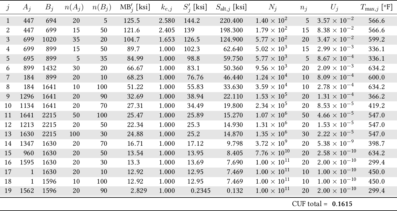
Figure 21: Results of the same fatigue problem solved using two different philosophies.. a — A multi-billion-dollar agency using the Windows philosophy (presumably mouse-based copy and pasted into Word), b — A small third-world consulting company using the Unix philosophy (FeenoX+AWK+LaTeX)
It should be noted that all of the programs and tools mentioned to be interoperable with FeenoX are free and open source software. This is not a requirement from the SRS, but is indeed a nice-to-have feature.
3 Interfaces
The tool should be able to allow remote execution without any user intervention after the tool is launched. To achieve this goal it is required that the problem should be completely defined in one or more input files and the output should be complete and useful after the tool finishes its execution, as already required. The tool should be able to report the status of the execution (i.e. progress, errors, etc.) and to make this information available to the user or process that launched the execution, possibly from a remote location.
FeenoX is provided as a console-only executable (recall it is a program, not a library) which can be run remotely through the mechanisms discussed in sec. 2.2 without any requirement such as graphical servers or special input devices. As already explained, when executed without any arguments, FeenoX writes a brief message with the version (further discussed in sec. 4.1) and the basic usage on the standard output and return to the calling shell with a return errorlevel zero:
$ feenox
FeenoX v0.3.292-gc932cb5
a cloud-first free no-fee no-X uniX-like finite-element(ish) computational engineering tool
usage: feenox [options] inputfile [replacement arguments] [petsc options]
-h, --help display options and detailed explanations of command-line usage
-v, --version display brief version information and exit
-V, --versions display detailed version information
--pdes list the types of PROBLEMs that FeenoX can solve, one per line
--elements_info output a document with information about the supported element types
--linear force FeenoX to solve the PDE problem as linear
--non-linear force FeenoX to solve the PDE problem as non-linear
Run with --help for further explanations.
$ echo $?
0
$ The --version option follows the GNU
Coding Standards guidelines:
$ feenox --version
FeenoX v0.3.292-gc932cb5
a cloud-first free no-fee no-X uniX-like finite-element(ish) computational engineering tool
Copyright © 2009--2024 https://seamplex.com/feenox
GNU General Public License v3+, https://www.gnu.org/licenses/gpl.html.
FeenoX is free software: you are free to change and redistribute it.
There is NO WARRANTY, to the extent permitted by law.
$The --versions option shows more information about the
FeenoX build and the libraries the binary was linked against:
$ feenox -V
FeenoX v1.0.8-g731ca5d
a cloud-first free no-fee no-X uniX-like finite-element(ish) computational engineering tool
Last commit date : Wed Mar 20 08:11:05 2024 -0300
Build date : Wed Mar 20 16:38:10 2024 -0300
Build architecture : linux-gnu x86_64
Compiler version : gcc (Debian 12.2.0-14) 12.2.0
Compiler expansion : gcc -Wl,-z,relro -I/usr/include/x86_64-linux-gnu/mpich -L/usr/lib/x86_64-linux-gnu -lmpich
Compiler flags : -O3 -flto=auto -no-pie
Builder : gtheler@tom
GSL version : 2.7.1
SUNDIALS version : N/A
PETSc version : Petsc Development GIT revision: v3.20.5-935-g78ad52f83fb GIT Date: 2024-03-25 05:31:58 +0000
PETSc arch : arch-linux-c-debug
PETSc options : --download-eigen --download-hdf5 --download-hypre --download-metis --download-mumps --download-parmetis --download-scalapack --download-slepc --with-64-bit-indices=no --with-debugging=yes --with-precision=double --with-scalar-type=real PETSC_ARCH=arch-linux-c-debug
SLEPc version : SLEPc Development GIT revision: v3.20.1-36-g7a35a7b97 GIT Date: 2023-12-02 02:30:03 -0600
$The --help option gives a more detailed usage:
$ feenox --help
usage: feenox [options] inputfile [replacement arguments] [petsc options]
-h, --help display options and detailed explanations of command-line usage
-v, --version display brief version information and exit
-V, --versions display detailed version information
-c, --check validates if the input file is sane or not
--pdes list the types of PROBLEMs that FeenoX can solve, one per line
--elements_info output a document with information about the supported element types
--linear force FeenoX to solve the PDE problem as linear
--non-linear force FeenoX to solve the PDE problem as non-linear
--progress print ASCII progress bars when solving PDEs
--mumps ask PETSc to use the direct linear solver MUMPS
Instructions will be read from standard input if “-” is passed as
inputfile, i.e.
$ echo 'PRINT 2+2' | feenox -
4
The optional [replacement arguments] part of the command line mean that
each argument after the input file that does not start with an hyphen
will be expanded verbatim in the input file in each occurrence of $1,
$2, etc. For example
$ echo 'PRINT $1+$2' | feenox - 3 4
7
PETSc and SLEPc options can be passed in [petsc options] (or [options])
as well, with the difference that two hyphens have to be used instead of
only once. For example, to pass the PETSc option -ksp_view the actual
FeenoX invocation should be
$ feenox input.fee --ksp_view
For PETSc options that take values, en equal sign has to be used:
$ feenox input.fee --mg_levels_pc_type=sor
See https://www.seamplex.com/feenox/examples for annotated examples.
Report bugs at https://github.com/seamplex/feenox/issues
Ask questions at https://github.com/seamplex/feenox/discussions
Feenox home page: https://www.seamplex.com/feenox/
$The input file provided as the first argument to the
feenox binary contains all the information needed to solve
the problem, so any further human intervention is not needed after
execution begins, as requested by the SRS. If the execution finishes
successfully, FeenoX returns a zero errorlevel to the calling shell (and
follows the Unix rule of silence, i.e. no PRINT
no output):
$ feenox maze.fee
$ echo $?
0
$If there is problem during execution (including parsing and run-time
errors), a line prefixed with error: is written into the
standard error file descriptor and a non-zero errorlevel is
returned:
$ feenox hello.fee
error: input file needs at least one more argument in commandline
$ echo $?
1
$ feenox hello.fee world
Hello world!
$ echo $?
0
$
This way, the error line can easily be parsed with standard Unix
tools like grep and cut or with a proper
regular expression parser. Eventually, any error should be forwarded
back to the initiating entity—which depending on the workflow can be a
human or an automation script—in order for her/him/it to fix it.
Following the rule of repair (sec. 11.12), ill-defined input files with missing material properties or inconsistent boundary conditions are detected before the actual assembly of the matrix begins:
$ feenox thermal-1d-dirichlet-no-k.fee
error: undefined thermal conductivity 'k'
$ feenox thermal-1d-dirichlet-wrong-bc.fee
error: boundary condition 'xxx' does not have a physical group in mesh file 'slab.msh'
$
Error code are designed to be useful and helpful. An attempt to open a file might fail due to a wide variety of reasons. FeenoX clearly states which one caused the error so it can be remedied:
$ cat test.fee
READ_MESH cantilever.msh
$ feenox test.fee
$ chmod -r cantilever.msh
$ feenox test.fee
error: 'Permission denied' when opening file 'cantilever.msh' with mode 'r'
$ rm cantilever.msh
$ feenox test.fee
error: 'No such file or directory' when opening file 'cantilever.msh' with mode 'r'
$
If the command-line option --progress (or the
PROGRESS keyword in PROBLEM)
is used, then FeenoX writes into the standard output three “bars”
showing the progress of
- (
.) the build and assembly of the problem matrices (stiffness and mass if applicable) - (
-) the iterative solution of the problem (either linear or non-linear) - (
=) the recovery of gradient-based (i.e. strains and stresses) out of the primary solution
Once again, these ASCII-based progress bars can be parsed by the calling entity and then present it back to the user. For example, fig. 10 shows how the web-based GUI CAEplex shows progress inside an Onshape tab.
Since FeenoX uses PETSc (and SLEPc), command-line options can be
passed from FeenoX to PETSc. The only difference is that since FeenoX
follows the POSIX standard regarding options and PETSc does not, double
dashes are required instead of PETSc’ single-dash approach. That is to
say, instead of -ksp_monitor one would have to pass
--ksp_monitor (see sec. 3.1.3 for details about the input
files):
$ feenox thermal-1d-dirichlet-uniform-k.fee --ksp_monitor
  0 KSP Residual norm 1.913149816332e+00
  1 KSP Residual norm 2.897817223901e-02
  2 KSP Residual norm 3.059845525572e-03
  3 KSP Residual norm 1.943995979588e-04
  4 KSP Residual norm 7.418444674938e-06
  5 KSP Residual norm 1.233527903582e-07
0.5
$
Any PETSc command-line option takes precedence over the settings in
the input file, so the pre-conditioner can be changed even if explicitly
given with the PRECONDITIONER
keyword:
$ feenox thermal-1d-dirichlet-uniform-k.fee --ksp_monitor --pc_type=ilu
  0 KSP Residual norm 2.678619047193e+00
  1 KSP Residual norm 7.172418823644e-16
0.5
$
If PETSc is compiled with MUMPS, FeenoX provides a
--mumps option:
$ feenox thermal-1d-dirichlet-uniform-k.fee --ksp_monitor --mumps
  0 KSP Residual norm 1.004987562109e+01
  1 KSP Residual norm 4.699798436762e-15
0.5
$
An illustration of the usage of PETSc arguments and the fact that
FeenoX automatically detects whether a problem is linear or not is given
below. The case thermal-1d-dirichlet-uniform-k.fee is
linear while the two-squares.fee from section sec. 2.5 is
not. Therefore, an SNES monitor should give output for the latter but
not for the former. In effect:
$ feenox thermal-1d-dirichlet-uniform-k.fee --snes_monitor
0.5
$ feenox two-squares.fee --snes_monitor
  0 SNES Function norm 9.658033489479e+00
  1 SNES Function norm 1.616559951959e+00
  2 SNES Function norm 1.879821597500e-01
  3 SNES Function norm 2.972104258103e-02
  4 SNES Function norm 2.624028350822e-03
  5 SNES Function norm 1.823396478825e-04
  6 SNES Function norm 2.574514225532e-05
  7 SNES Function norm 2.511975376809e-06
  8 SNES Function norm 4.230090605033e-07
  9 SNES Function norm 5.154440365087e-08
$
As already explained in sec. 2.2.2, FeenoX supports run-time
replacement arguments that get replaced verbatim in the input file. This
feature is handy when the same problem has to be solved over different
meshes, such as when investigating the h-convergence order over Gmsh’s element scale
factor -clscale:
PROBLEM thermal 1D
READ_MESH slab-$1.msh
k(x) = 1+T(x)
BC left  T=0
BC right T=1
SOLVE_PROBLEM
PRINT nodes %+.2e integral((T(x)-(sqrt(1+(3*x))-1))^2,x,0,1)
$ for c in $(feenox steps.fee); do gmsh -v 0 -1 slab.geo -clscale ${c} -o slab-${c}.msh; feenox thermal-1d-dirichlet-temperature-k-parametric.fee ${c}; done | sort -g
11 +6.50e-07
13 +3.15e-07
14 +2.29e-07
15 +1.70e-07
17 +1.00e-07
20 +5.04e-08
24 +2.34e-08
32 +7.19e-09
39 +3.46e-09
49 +1.31e-09
$Since the main input file is the first argument (not counting POSIX
options starting with at least one dash), FeenoX might be invoked
indirectly by adding a shebang line
to the input file with the location of the system-wide executable and
setting execution permissions on the input file itself. So if we modify
the above hello.fee example as hello
#!/usr/local/bin/feenox
PRINT "Hello $1!"
and then we can do
$ chmod +x hello
$ ./hello world
Hello world!
$ ./hello universe
Hello universe!
$
For example, the following she-banged input file can be used to compute the derivative of a column with respect to the other as a Unix filter:
#!/usr/local/bin/feenox
FUNCTION f(t) FILE - INTERPOLATION steffen

a = vecmin(vec_f_t)
b = vecmax(vec_f_t)

# time step from arguments (or default 10 steps)
DEFAULT_ARGUMENT_VALUE 1 (b-a)/10
h = $1

VAR t'
f'(t) = derivative(f(t'),t',t)

PRINT_FUNCTION f' MIN a+0.5*h MAX b-0.5*h STEP h
$ feenox f.fee "sin(t)" 1 | ./derivative.fee
0.05 0.998725
0.15 0.989041
0.25 0.968288
0.35 0.939643
0.45 0.900427
0.55 0.852504
0.65 0.796311
0.75 0.731216
0.85 0.66018
0.95 0.574296
$where f.fee is a “command-line function generator”:
end_time = $2
PRINT t $1
3.1 Problem input
The problem should be completely defined by one or more input files. These input files might be
- particularly formatted files to be read by the tool in an ad-hoc way, and/or
- source files for interpreted languages which can call the tool through and API or equivalent method, and/or
- any other method that can fulfill the requirements described so far.
Preferably, these input files should be plain ASCII files in order to allow to manage changes using distributed version control systems such as Git. If the tool provides an API for an interpreted language such as Python, then the Python source used to solve a particular problem should be Git-friendly. It is recommended not to track revisions of mesh data files but of the source input files, i.e. to track the mesher’s input and not the mesher’s output. Therefore, it is recommended not to mix the problem definition with the problem mesh data.
It is not mandatory to include a GUI in the main distribution, but the input/output scheme should be such that graphical pre and post-processing tools can create the input files and read the output files so as to allow third parties to develop interfaces. It is recommended to design the workflow as to make it possible for the interfaces to be accessible from mobile devices and web browsers.
It is expected that 80% of the problems need 20% of the functionality. It is acceptable if only basic usage can be achieved through the usage of graphical interfaces to ease basic usage at first. Complex problems involving non-trivial material properties and boundary conditions not be treated by a GUI and only available by needing access to the input files.
FeenoX currently works by reading an input file (which in turn can
recursively INCLUDE
further input files) with an ad-hoc format, whose rationale is
described in this section. Therefore, it already does satisfy
requirement a. but, eventually, could also satisfy requirement b. by
adding a wrapper for high-level languages such as
- Python
- Julia
- R
that would either
- create an input file and run FeenoX in the back, or
- successively call the FeenoX functions that define definitions and execute instructions (to be done).
As already explained in sec. 1, the motto is “FeenoX is—in a certain sense—to desktop FEA programs and libraries what Markdown is to Word and (La)TeX, respectively and deliberately.” Hence, the input files act as the Markdown source: instructions about what to do but not how to do it.
The input files are indeed plain-text ASCII files with English-like keywords that fully define the problem. The main features of the input format, thoroughly described below, are:
- It is syntactically sugared by using English-like keywords.
- Nouns are definitions and verbs are instructions.
- Simple problems need simple inputs.
- Simple things should be simple, complex things should be possible.
- Whenever a numerical value is needed an expression can be given (i.e. “everything is an expression.”)
- The input file should match as much as possible the paper (or blackboard) formulation of the problem.
- It provides means to compare numerical solutions against analytical ones.
- It should be possible to read run-time arguments from the command line.
- Input files are distributed version control-friendly.
3.1.1 Syntactic sugar & highlighting
The ultimate goal of FeenoX is to solve mathematical equations that are hard to solve with pencil and paper. In particular, to integrate differential equations (recall that the first usable computer was named ENIAC, which stands for Electronic Numerical Integrator and Computer). The input file format was designed as to how to ask the computer what to compute. The syntax, based on keywords and alphanumerical arguments was chosen as to sit in the middle of the purely binary numerical system employed by digital computers6 and the purely linguistical nature of human communication. The rationale behind its design is that an average user can peek a FeenoX input file and tell what it is asking the computer to compute, as already illustrated for the NAFEMS LE10 problem in fig. 3. Even if the input files are created by a computer and not by a human, the code used to create a human-friendly input file will be human-friendlier than a code that writes only zeroes and ones as its output (that will become the input of another one following the Unix rule of composition sec. 11.3). As an exercise, compare the input file in fig. 3 (or in fig. 22) with the inputs files used by other open source FEA solvers shown in appendix sec. 14.
The first argument not starting with a dash to the
feenox executable is the path to the main input file. This
main input file can in turn include other FeenoX input files (with the
INCLUDE
keyword) and/or read data from other files (such as meshes with the READ_MESH
instruction) or other resources (such as data files for point-wise data
interpolation with FUNCTION
or shared memory objects TBD).
For instance, the test
directory includes some spinning-disk
cases that compare the analytical solution for the hoop and radial
stresses with the numerical ones obtained with FeenoX. These cases read
the radius R and thickness t from the .geo file used by
Gmsh to build the mesh in the first place:
# analytical solution
INCLUDE spinning-disk-dimensions.geo
S_h(r) = ((3+nu)*R^2 - (1+3*nu)*r^2)
S_r(r) = (3+nu) * (R^2 - r^2)
where spinning-disk-dimensions.geo is
R = 0.1;
t = 0.003;
The input files are plain text files, either pure ASCII or UTF-8
(more details in sec. 3.1.9). In principle any extension (even no
extension) can be used for the FeenoX input files. Throughout the FeenoX
repository and documentation the extension .fee is used,
which has a couple of advantages:
The
.feeextension is detected by syntax-highlighting extensions for common editors (both graphical such as Kate and cloud-friendly such as Vim) as illustrated in fig. 22.The expression
$0(or${0}) is expanded to the base name of the input file, i.e. the directory part (if present) is removed and the.feeextension is removed. Therefore,READ_MESH $0.mshwould read a mesh file whose name is the same as the FeenoX input file, without the
.feeextension.
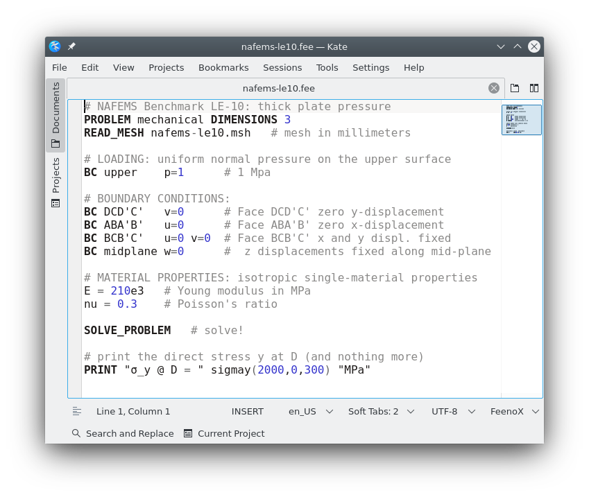
Figure 22: Syntax highlighting of input files in GUI and cloud-friendly text editors. a — Kate, b — Vim
3.1.2 Definitions and instructions
The way to tell the computer what problem it has to solve and how to solve it is by using keywords in the input file. Each non-commented line of the input file should start with either
- a primary keyword such as
PROBLEMorREAD_MESH, or - a variable such as
end_timeor a vector or matrix with the corresponding index(es) such asv[2]orA[i][j]followed by the=keyword, or - a function name with its arguments such as
f(x,y)followed by the=keyword.
A primary keyword usually is followed by arguments and/or secondary keywords, which in turn can take arguments as well. For example, in
PROBLEM mechanical DIMENSIONS 3
READ_MESH $0.msh
[...]
# print the direct stress y at D (and nothing more)
PRINT "σ_y @ D = " sigmay(2000,0,300) "MPa"
we have PROBLEM
acting as a primary keyword, taking mechanical as its first
argument and then DIMENSIONS as a secondary keyword with
3 being an argument to the secondary keyword. Then
READ_MESH is another primary keyword taking
$0.msh (which would be expanded to something like
nafems-le10.msh) as its argument.
A primary keyword can be
- a definition,
- an instruction, or
- both.
Definitions are English nouns and instructions are English
verbs. In the example above, PROBLEM
is a definition because it tells FeenoX about something it has to do
(i.e. that it has to solve a three-dimensional problem), but does not do
anything actually. On the other hand, READ_MESH
is both a definition and an instruction: it defines that there exists a
mesh named nafems-le10.msh which might be referenced later
(for example in an INTEGRATE
or WRITE_MESH
instructions), but it also asks FeenoX to read the mesh at that point of
the instruction list (more details below). Finally, PRINT
is a primary keyword taking different types and number or arguments. It
is an instruction because it does not define anything, it just asks
FeenoX to print the value of the function named sigmay
evaluated at 2000,0,300. In this case,
sigmay is a function which is implicitly defined when PROBLEM
is set to mechanical. If sigmay was referenced
before PROBLEM,
FeenoX would not find it. And if the problem was of any other type,
FeenoX would not find it even when referenced from the last line of the
input file.
The following example further illustrates the differences between definitions and instructions. It compares the result of (numerically but adaptively) integrating f(x,y,z) = \sin(x^3 + y^2 + z) over a unit cube against using a 3D Gauss integration scheme over a fixed set of quadrature points on the same unit cube meshes with two regular hexahedra in each direction (totaling 8 hexahedra). In one case hex20 are used and in the other one, hex27. Both cases use 27 quadrature points per element.
# these two are instructions to read a two meshes
# but they also define two mesh names that can be referred to later
READ_MESH hex20.msh DIM 3
READ_MESH hex27.msh DIM 3

# these three lines are definitions, they define three functions
# the first two also define four vectors for each function
#  1. vec_f20_x and vec_f27_x with the x coordinates of the mesh' nodes
#  2. vec_f20_y and vec_f27_y with the y coordinates of the mesh' nodes
#  3. vec_f20_z and vec_f27_z with the z coordinates of the mesh' nodes
#  4. vec_f20 and vec_f27 with the value of the function at the i-th node
# these definitions do not evaluate the functions, but they fill vectors 1-3
# (we'll fill vectors 4 below)
# note that these definitions refer to the meshes defined above in READ_MESH
FUNCTION f20(x,y,z) MESH hex20.msh
FUNCTION f27(x,y,z) MESH hex27.msh
f(x,y,z) = sin(x^3 + y^2 + z)

# these two lines are assignment instructions, they "fill" in
# the vectors with the value of the functinos f20(x,y,z) and f27(x,y,z)
# by evaluating f(x,y,z) at the nodes of the two meshes
# (there is a implicit loop for the index i over the size of the vectors)
vec_f20[i] = f(vec_f20_x[i], vec_f20_y[i], vec_f20_z[i])
vec_f27[i] = f(vec_f27_x[i], vec_f27_y[i], vec_f27_z[i])

# this line is an assignment, that first defines a variable If0
# and then calls the functional integral three times to perform a
# "continuous" (in the sense that it is numeric but adaptive) triple integration
If0 = integral(integral(integral(f(x,y,z), z, 0, 1), y, 0, 1), x, 0, 1)

# these two lines are instructions, they integrate functions f20 and f27 over
# each of the meshes and then they store the results in the (implicitly defined)
# variables If20 and If27
INTEGRATE f20  MESH hex20.msh RESULT If20
INTEGRATE f27  MESH hex27.msh RESULT If27

# these lines are instructions, they print stuff to the standard output
# nothing is defined
PRINT %.10f If0
PRINT %.10f If20  %+.2e If20-If0
PRINT %.10f If27  %+.2e If27-If0
$ $ feenox integral_over_hex.fee
0.7752945175
0.7753714586 +7.69e-05
0.7739155101 -1.38e-03
$3.1.3 Simple inputs
Consider solving heat conduction on a one-dimensional slab spanning the unitary range x \in [0,1]. The slab has a uniform unitary conductivity k=1 and Dirichlet boundary conditions
\begin{cases} T(0) &= 0 \\ T(1) &= 1 \end{cases}
This simple problem has the following simple input:
PROBLEM thermal 1D               # tell FeenoX what we want to solve
READ_MESH slab.msh               # read mesh in Gmsh's v4.1 format
k = 1                            # set uniform conductivity
BC left  T=0                     # set fixed temperatures as BCs
BC right T=1                     # "left" and "right" are defined in the mesh
SOLVE_PROBLEM                    # tell FeenoX we are ready to solve the problem
PRINT T(0.5)                     # ask for the temperature at x=0.5
$ feenox thermal-1d-dirichlet-uniform-k.fee
0.5
$Now, if instead of having a uniform conductivity the problem had a space-dependent k(x) = 1+x then the input would read
PROBLEM thermal 1D
READ_MESH slab.msh
k(x) = 1+x                       # space-dependent conductivity
BC left  T=0
BC right T=1
SOLVE_PROBLEM
PRINT T(1/2) log(1+1/2)/log(2)   # print numerical and analytical solutions
$ feenox thermal-1d-dirichlet-space-k.fee
0.584893 0.584963
$Finally, if the conductivity depended on temperature (rendering the problem non-linear) say like k(x) = 1 + T(x) then
PROBLEM thermal 1D
READ_MESH slab.msh
k(x) = 1+T(x)                    # temperature-dependent conductivity
BC left  T=0
BC right T=1
SOLVE_PROBLEM
PRINT T(1/2) sqrt(1+(3*0.5))-1   # print numerical and analytical solutions
$ feenox thermal-1d-dirichlet-space-k.fee
0.581139 0.581139
$Note that FeenoX could figure out by itself that the two first cases
were linear while the last one was not. This can be verified by passing
the extra argument --snes_view. In the first two cases,
there will be no extra output. In the last one, the details of the
non-linear solver used by PETSc will be written into the standard
output. The experienced reader should take some time to compare the
effort and level of complexity that other FEA solvers require in order
to set up simple problems like these. A discussion of the difference
between linear and non-linear problems can be found in the heat
conduction tutorial.
3.1.4 Complex things
Alan Kay’s idea that “simple things should be simple, complex things should be possible” has already been mentioned in sec. 2.5. The first part of the quote was addressed in the previous section. Of course, complexity can scale up almost indefinitely so we cannot show an example right here. But the following repositories contain the scripts and input files (for Gmsh, FeenoX and other common Unix tools such as Sed and Awk) that solve non-trivial problems using FeenoX as the main tool and employing free and open source software only, both for the computation and for the creation of figures and result tables.
Convergence study on stress linearization of an infinite pipe according to ASME: a parametric study over the number of elements through the thickness of a pipe and the error committed when computing membrane and bending stresses according to ASME VIII Div 2 Sec 5. The study uses the following element types
- unstructured tet4
- unstructured straight tet10
- unstructured curved tet10
- structured straight tet10
- structured curved tet10
- structured hex8
- structured straight hex20
- structured curved hex20
- structured straight hex27
- structured curved hex27
The linearized stresses for different number of elements through the pipe thickness are compared against the analytical solution. Figures with the meshes employed in each case and with plots of profiles vs. the radial coordinate and linearized stresses vs. number of elements through the thickness are created.
Environmentally-assisted fatigue analysis of dissimilar material interfaces in piping systems of a nuclear power plant: a case that studies environmentally-assisted fatigue using environment factors applied to traditional in-air ASME fatigue analysis for operational an incidental transients in nuclear power plant as propose by EPRI. A fictitious CAD geometry representing a section of a piping system is studied. Four operational transients are made up with time-dependent data for pressure and water temperature.
- A transient heat conduction problem with temperature-dependent material properties (according to ASME property tables) are solved over a small region around a material interface between carbon and stainless steel.
- Primary stresses according to ASME are computed for each of the operational transients.
- The results of a modal analysis study are convoluted with a frequency spectrum of a design-basis earthquake using the SRSS method to obtain an equivalent static volumetric force distribution.
- The time-dependent temperature distribution for each transient is then used in quasi-static mechanical problems to compute secondary stresses according to ASME, including the equivalent seismic loads at the moment of higher thermal stresses.
- The history of linearized Tresca stresses are juxtaposed to compute the cumulative usage factors using the ASME peak-valley method.
- Environmental data is used to affect each cumulative usage factors with an environment factor to account for in-water conditions.
These repositories contain a run.sh that, when executed
in a properly-set-up GNU/Linux host (either on premises or in the
cloud), will perform a number of steps including
- creation of appropriate meshes
- execution FeenoX
- generation post-processing views, plots or tables with the results
- etc.
Refer to the READMEs in each repository for further details about the mathematical models involved.
3.1.5 Everything is an expression
As explained in the history of FeenoX (sec. 12), the first objective of the code was to solve ODEs written in an ASCII file as human-friendly as possible. So even before any other feature, the first thing the FeenoX ancestors had was an algebraic parser and evaluator. This was back in 2009, and I performed an online search before writing the whole thing from scratch. I found a nice post in Slack Overflow7 that discussed some cool ideas and even had some code published under the terms of the Creative Commons license.
Besides ODEs, algebraic expressions are a must if one will be dealing with arbitrary functions in general and spatial distributions in particular—which is essentially what PDE solvers are for. If a piece of software wants to allow features ranging from comparing numerical results with analytical expression to converting material properties from a system of units to another one in a straightforward way for the user (either an actual human being or a computer creating an input file), it ought to be able to handle algebraic expressions.
Appropriately handling algebraic expressions leads to fulfilling the Unix rule of least surprise (sec. 11.10). If the user needs to define a function f(x) = 1/2 \cdot x^2, all she has to do is write
f(x) = 1/2 * x^2And conversely, if someone reads the line above, she can rest assure that there’s a function called f(x) that will evaluate to 1/2 \cdot x^2 when needed. In effect, anyone can expect the output of this instruction
PRINT integral(f(x), x, 0, 1)to be one third.
Of course, expressions are needed to get 100%-user defined output
(further discussed in sec. 3.2), as with the PRINT
instruction above. But once an algebraic parser and evaluator is
available, it does not make sense to keep force the user to write
numerical data only. What if a the angular speed is in RPM and the model
needs it in radians per second? Instead of having to write
104.72, FeenoX allows the user to write
w = 1000 * 60*pi/180This way,
- it is easy to see what the speed in RPM is
- precision is not lost
- should the speed change, it is trivial to change the
1000for anything else.
Whenever an input keyword needs a numerical value, any expression will do:
n = 3
VECTOR x SIZE 2+n
x[i] = i^2
PRINT x
$ feenox vector_size_one_plus_n.fee
1 4 9 16 25
$It goes without saying that algebraic expressions are a must when defining transient and/or space-dependent boundary conditions for PDEs:
PROBLEM thermal 1D
READ_MESH slab.msh

end_time = 10
k = 1
kappa = 0.1

FUNCTION f(t) DATA {
0    0
1    1
2    1
3    2
4    0
10   0
}
BC left  T=f(t)

w = 0.5*pi
BC right T=1+sin(w*t)

SOLVE_PROBLEM
PRINT t T(0) T(0.5) T(1)
Besides purely algebraic expressions, FeenoX can handle point-wise defined functions which can then be used in algebraic expressions. A useful example is allowing material properties (e.g. Young modulus) to depend on temperature. Consider a simple plane-strain square [-1,+1]\times[-1,+1] fixed on one side and with a uniform tension in the opposite one while leaving the other two free. The square’s Young modulus depends on temperature according to a one-dimensional point-wise defined function E_\text{carbon}(T) given by pairs stated according to one of the many material properties tables from ASME II and interpolated using Steffen’s method. Although in this example the temperature is given as an algebraic expression of space, in particular
T(x,y)~[\text{ºC}] = 200 + 350 \cdot y
PROBLEM mechanical plane_strain
READ_MESH square-centered.msh # [-1:+1]x[-1:+1]

# fixed at left, uniform traction in the x direction at right
BC left    fixed
BC right   tx=50

# ASME II Part D pag. 785 Carbon steels with C<=0.30%
FUNCTION E_carbon(temp) INTERPOLATION steffen DATA {
-200  216
-125  212
-75   209
25    202
100   198
150   195
200   192
250   189
300   185
350   179
400   171
450   162
500   151
550   137
}


# known temperature distribution
# (we could have read it from an output of a thermal problem)
T(x,y) := 200 + 350*y

# Young modulus is the function above evaluated at the local temperature
E(x,y) := E_carbon(T(x,y))

# uniform Poisson's ratio
nu = 0.3

SOLVE_PROBLEM
WRITE_MESH mechanical-square-temperature.vtk  E  VECTOR u v 0
By replacing T(x,y) = 200 + 350*y with
T(x,y) = 200 we can compare the results of the
temperature-dependent case with the uniform-properties case
(fig. 23):
$ feenox mechanical-square-temperature.fee
$ diff mechanical-square-temperature.fee mechanical-square-uniform.fee
29c29
< T(x,y) := 200 + 350*y
---
> T(x,y) := 200
38c38
< WRITE_MESH mechanical-square-temperature.vtk  E  VECTOR u v 0
---
> WRITE_MESH mechanical-square-uniform.vtk  E  VECTOR u v 0
$ feenox mechanical-square-uniform.fee
$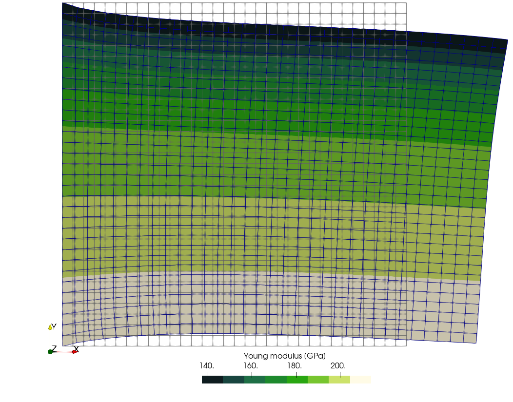
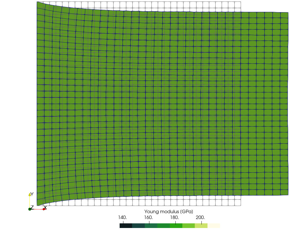
Figure 23: Mechanical plane-strain square with temperature-dependent Young modulus and comparison with uniform reference case.. a — Temperature-dependent E, b — Uniform E for reference
In real applications this distribution T(x,y) can be read from the output of an actual heat conduction problem. See sec. 3.2.2 for a revisit of this case, reading the temperature from an unstructured triangular mesh instead of hard-coding it as an algebraic expression of space.
So remember, in FeenoX everything is an expression—especially temperature, as also shown in the next section.
3.1.6 Matching formulations
The Lorenz’
dynamical system system and the NAFEMS LE10
benchmark problem, both discussed earlier in sec. 1.2, illustrate how
well the FeenoX input file matches the usual human-readable formulation
of ODE or PDE problems. In effect, fig. 3 shows there is a trivial
one-to-one correspondence between the sections of the problem formulated
in a sheet of paper and the text file nafems-le10.fee. The
same effect can be seen in the NAFEMS LE11 problem, which involves a
temperature distribution given as an algebraic expression of \vec{x}:
Let us consider the NAFEMS LE11 benchmark problem titled “Solid cylinder/taper/sphere-temperature” stated in fig. 24. It consists of an axi-symmetrical geometry subject to thermal loading by a temperature distribution given by an algebraic expression. The material properties are linear, orthotropic and uniform. The boundary conditions prescribe symmetries in all directions.
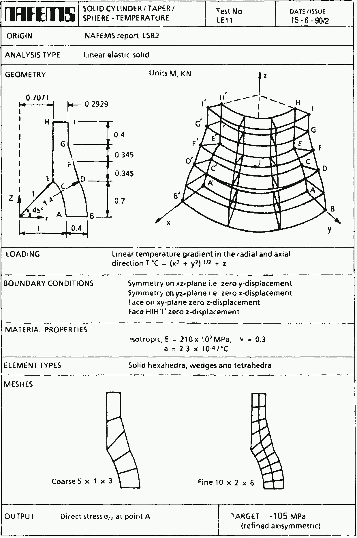
- Loading
Linear temperature gradient in the radial an axial direction
T(x,y,z)~\text{[ºC]} = \left(x^2+ y^2\right)^{1/2} + z
- Boundary conditions
- Symmetry on x-z plane, i.e. zero y-displacement
- Symmetry on y-z plane, i.e. zero x-displacement
- Face on x-y plane zero z-displacement
- Face HIH'I' zero z-displacement
- Material properties
- Isotropic, E=210 \times 10^3~\text{MPa}, \nu = 0.3
- Thermal expansion coefficient \alpha = 2.3 \times 10^{-4}~\text{ºC}^{-1}
- Output
- Direct stress \sigma_{zz} at point A
To solve this problem, we can use the following FeenoX input file that exactly matches the human-readable formulation:
PROBLEM mechanical
READ_MESH $0.msh

# linear temperature gradient in the radial and axial direction
T(x,y,z) = (x^2 + y^2)^(1/2) + z

# Boundary conditions
BC xz     symmetry
BC yz     symmetry
BC xy     w=0
BC HIH'I' w=0

# material properties (isotropic & uniform so we can use scalar constants)
E = 210e3*1e6       # mesh is in meters, so E=210e3 MPa -> Pa
nu = 0.3            # dimensionless
alpha = 2.3e-4      # in 1/ºC as in the problem

SOLVE_PROBLEM
WRITE_RESULTS FORMAT vtk
PRINT "sigma_z(A) =" sigmaz(0,1,0)/1e6 "MPa (target was -105 MPa)" SEP " "
$ time feenox nafems-le11.fee
sigma_z(A) = -105.041 MPa (target was -105 MPa)
real 0m1.766s
user 0m1.642s
sys 0m0.125s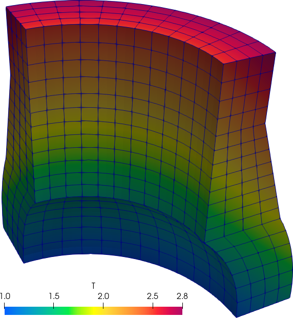
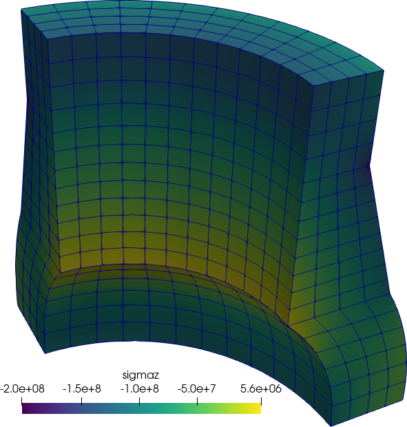
Figure 25: The NAFEMS LE11 problem results. a — Problem statement, b — Structured hex mesh

This feature can be better appreciated by comparing the input files needed to solve these kind of NAFEMS benchmarks with other finite-element tools. Sec. 14 gives a glimpse for the NAFEMS LE10 problem, where the input files are way too cryptic and cumbersome as compared to what FeenoX needs.
3.1.7 Comparison of solutions
One cornerstone design feature is that FeenoX has to provide a way to compare its numerical results with other already-know solutions—either analytical or numerical—in order to verify their validity. Indeed, being able to take the difference between the numerical result and an algebraic expression evaluated at arbitrary locations (usually quadrature points to compute~L_p norms of the error) is a must if code verification is required.
Let us consider a one-dimensional slab reactor with uniform macroscopic cross sections
\begin{aligned} \Sigma_t &= 0.54628~\text{cm}^{-1} \\ \Sigma_s &= 0.464338~\text{cm}^{-1} \\ \nu\Sigma_f &= 1.70 \cdot 0.054628~\text{cm}^{-1} \end{aligned}
such that, if computed with neutron transport theory, is exactly critical with a width of a = 2 \cdot 10.371065~\text{cm}. Just to illustrate a simple case, we can solve it using the diffusion approximation with zero flux at both as. This case has an analytical solution for both the effective multiplication factor
k_\text{eff} = \frac{\nu\Sigma_f}{(\Sigma_t - \Sigma_s) + D \cdot \left(\frac{\pi}{a} \right)^2}
and the flux distribution
\phi(x) = \frac{\pi}{2} \cdot \sin\left(\frac{x}{a} \cdot \pi\right)
provided the diffusion coefficient D is defined as
D = \frac{1}{3 \cdot \Sigma_t}
We can solve both the numerical and analytical problems in FeenoX, and more importantly, we can subtract them at any point of space we want:
PROBLEM neutron_diffusion 1D
READ_MESH slab-UD20-1-0-SL.msh

a = 2 * 10.371065 # critical size of the problem UD20-1-0-SL (number 22 report Los Alamos)

Sigma_t1 = 0.54628
Sigma_s1.1 = 0.464338
nuSigma_f1 = 1.70*0.054628
D1 = 1/(3*Sigma_t1)

# null scalar flux at both ends of the slab
BC left  null
BC right null

SOLVE_PROBLEM

# analytical effective multiplication factor (diffusion approximation)
keff_diff = nuSigma_f1/((Sigma_t1-Sigma_s1.1) + D1*(pi/a)^2)

# analytical normalized flux distribution (diffusion approximation)
phi_diff(x) = pi/2 * sin(x/a * pi)

PRINT_FUNCTION FORMAT %+.3f phi1 phi_diff phi1(x)-phi_diff(x) HEADER
PRINT TEXT "\# keff      = " %.8f keff
PRINT TEXT "\# kdiff     = " %.8f keff_diff
PRINT TEXT "\# rel error = " %+.2e (keff-keff_diff)/keff
$ feenox neutron-diffusion-1d-null.fee
# x phi1 phi_diff phi1(x)-phi_diff(x)
+0.000 +0.000 +0.000 +0.000
+10.371 +1.574 +1.571 +0.003
+20.742 +0.000 +0.000 -0.000
+1.474 +0.348 +0.348 +0.001
+2.829 +0.654 +0.653 +0.001
+4.074 +0.911 +0.909 +0.002
+5.217 +1.118 +1.116 +0.002
+6.268 +1.280 +1.277 +0.002
+7.233 +1.399 +1.397 +0.003
+8.120 +1.483 +1.480 +0.003
+8.935 +1.537 +1.534 +0.003
+9.683 +1.565 +1.562 +0.003
+11.059 +1.565 +1.562 +0.003
+11.807 +1.537 +1.534 +0.003
+12.622 +1.483 +1.480 +0.003
+13.509 +1.399 +1.397 +0.003
+14.474 +1.280 +1.277 +0.002
+15.525 +1.118 +1.116 +0.002
+16.668 +0.911 +0.909 +0.002
+17.913 +0.654 +0.653 +0.001
+19.268 +0.348 +0.348 +0.001
# keff = 0.96774162
# kdiff = 0.96797891
# rel error = -2.45e-04
$Something similar could have been done for two groups of energy, although the equations get a little bit more complex so we leave it as an example in the Git repository.
A notable non-trivial thermo-mechanical problem that nevertheless has an analytical solution for the displacement field is the “Parallelepiped whose Young’s modulus is a function of the temperature” (fig. 27). The problem consists of finding the non-dimensional temperature T and displacements u, v and w distributions within a solid parallelepiped of length \ell whose base is a square of h\times h. The solid is subject to heat fluxes and to a traction pressure at the same time. The non-dimensional Young’s modulus E of the material depends on the temperature T in a know algebraically way, whilst both the Poisson coefficient \nu and the thermal conductivity k are uniform and do not depend on the spatial coordinates:
\begin{aligned} E(T) &= \frac{1000}{800-T} \\ \nu &= 0.3 \\ k &= 1 \end{aligned}

The thermal boundary conditions are
- Temperature at point A at (\ell,0,0) is zero
- Heat flux q^{\prime \prime} through x=\ell is +2
- Heat flux q^{\prime \prime} through x=0 is -2
- Heat flux q^{\prime \prime} through y=h/2 is +3
- Heat flux q^{\prime \prime} through y=-h/2 is -3
- Heat flux q^{\prime \prime} through z=h/2 is +4
- Heat flux q^{\prime \prime} through z=-h/2 is -4
The mechanical boundary conditions are
- Point O at (0,0,0) is fixed
- Point B at (0,h/2,0) is restricted to move only in the y direction
- Point C at (0,0,/h2) cannot move in the x direction
- Surfaces x=0 and x=\ell are subject to an uniform normal traction equal to one
The analytical solution is
\begin{aligned} T(x,y,z) &= -2x -3y -4z + 40 \\ u(x,y,z) &= \frac{A}{2} \cdot\left[x^2 + \nu\cdot\left(y^2+z^2\right)\right] + B\cdot xy + C\cdot xz + D\cdot x - \nu\cdot \frac{Ah}{4} \cdot \left(y+z\right) \\ v(x,y,z) &= -\nu\cdot \left[A\cdot x y + \frac{B}{2} \cdot \left(y^2-z^2+\frac{x^2}{\nu}\right) + C\cdot y z + D\cdot y -A\cdot h/4\cdot x - C\cdot h/4\cdot z\right] \\ w(x,y,z) &= -\nu\cdot \left[A\cdot x z + B\cdot yz + C/2\cdot \left(z^2-y^2+\frac{x^2}{\nu}\right) + D\cdot z + \frac{Ch}{4} \cdot y - \frac{Ah}{4} \cdot x\right] \\ \end{aligned}
where~A=0.002, B=0.003, C=0.004 and~D=0.76. The reference results are the temperature at points O and D and the displacements at points A and D (tbl. 2}.
| Point | Unknown | Reference value |
|---|---|---|
| O | T | +40.0 |
| D | T | -35.0 |
| A | u | +15.6 |
| v | -0.57 | |
| w | -0.77 | |
| D | u | +16.3 |
| v | -1.785 | |
| w | -2.0075 |
First, the thermal problem is solved with FeenoX and the temperature
distribution T(x,y,z) is written into a
.msh file.
PROBLEM neutron_diffusion 1D
READ_MESH slab-UD20-1-0-SL.msh

a = 2 * 10.371065 # critical size of the problem UD20-1-0-SL (number 22 report Los Alamos)

Sigma_t1 = 0.54628
Sigma_s1.1 = 0.464338
nuSigma_f1 = 1.70*0.054628
D1 = 1/(3*Sigma_t1)

# null scalar flux at both ends of the slab
BC left  null
BC right null

SOLVE_PROBLEM

# analytical effective multiplication factor (diffusion approximation)
keff_diff = nuSigma_f1/((Sigma_t1-Sigma_s1.1) + D1*(pi/a)^2)

# analytical normalized flux distribution (diffusion approximation)
phi_diff(x) = pi/2 * sin(x/a * pi)

PRINT_FUNCTION FORMAT %+.3f phi1 phi_diff phi1(x)-phi_diff(x) HEADER
PRINT TEXT "\# keff      = " %.8f keff
PRINT TEXT "\# kdiff     = " %.8f keff_diff
PRINT TEXT "\# rel error = " %+.2e (keff-keff_diff)/keff
Then, the mechanical problem reads two meshes: one for solving the actual mechanical problem and another one for reading T(x,y,z) from the previous step. Note that the former contains second-order hexahedra and the latter first-order tetrahedra. After effectively solving the problem, it writes again tbl. 2 in Markdown.
3.1.8 Run-time arguments
The usage of run-time command-line arguments was illustrated
in sec. 2.2.2. The idea is that if the expression $n (or
${n}) is found in the input file, the FeenoX parser expands
the expression literally as the n-th
non-optional argument in the command line. The case n=0 is particular in the sense that, as
explained in sec. 3.1.1, expands to the name of the input file without
the leading directory path and the trailing extension
.fee.
The definition DEFAULT_ARGUMENT_VALUE
can be used to give a default value for arguments not provided.
otherwise, FeenoX would complain:
$ echo "PRINT \$1" | feenox -
error: input file needs at least one more argument in commandline
$ echo -e "DEFAULT_ARGUMENT_VALUE 1 hello\nPRINT \$1" | feenox -
hello
$
This feature is extensively used in parametric and optimization runs such as in the verification using the Method of Manufactured solutions:
# MMS data, set T_mms(x) and k_mms(x) as desired
T_mms(x,y) = 1 + sin(2*x)^2 * cos(3*y)^2
k_mms(x,y) = 1 + x - 0.5*y

READ_MESH square-$2-$3-$4.msh DIMENSIONS 2
PROBLEM thermal

DEFAULT_ARGUMENT_VALUE 1 dirichlet # BCs = dirichlet/neumann
DEFAULT_ARGUMENT_VALUE 2 tri3      # shape = tri3/tri6/quad4/quad8/quad9
DEFAULT_ARGUMENT_VALUE 3 struct    # algorithm = struct/frontal/delaunay
DEFAULT_ARGUMENT_VALUE 4 8         # refinement factor = 1/2/3/4...
DEFAULT_ARGUMENT_VALUE 5 0         # write vtk? = 0/1

# read the results of the symbolic derivatives
INCLUDE thermal-square-q.fee

# set the PDE coefficients and BCs we just read above
k(x,y) = k_mms(x,y)
q(x,y) = q_mms(x,y)

# set the BCs (depending on $1)
INCLUDE thermal-square-bc-$1.fee

SOLVE_PROBLEM   # this line should be self-explanatory

# output
PHYSICAL_GROUP bulk DIM 2
h = sqrt(bulk_area/cells)

# L-2 error
INTEGRATE (T(x,y)-T_mms(x,y))^2 RESULT e_2
error_2 = sqrt(e_2)

# L-inf error
FIND_EXTREMA abs(T(x,y)-T_mms(x,y)) MAX error_inf

PRINT %.6f log(h) log(error_inf) log(error_2) %g $4 cells nodes %.2f 1024*memory() wall_time()

IF $5
  WRITE_MESH thermal-square_$1-$2-$3-$4.vtk T q T_mms T(x,y)-T_mms(x,y)
ENDIF
which is called from a Bash loop that looks like
bcs="dirichlet neumann"
elems="tri3 tri6 quad4 quad8 quad9"
algos="struct frontal delaunay"
cs="4 6 8 10 12 16 20 24 30 36 48"

[...]

for bc in ${bcs}; do
 for elem in ${elems}; do
  for algo in ${algos}; do

    [...]

    for c in ${cs}; do

     name="thermal_square_${bc}-${elem}-${algo}-${c}"

     # prepare mesh
     if [ ! -e square-${elem}-${algo}-${c}.msh ]; then
       lc=$(echo "PRINT 1/${c}" | feenox -)
       gmsh -v 0 -2 square.geo ${elem}.geo ${algo}.geo -clscale ${lc} -o square-${elem}-${algo}-${c}.msh
     fi

     # run feenox
     feenox thermal-square.fee ${bc} ${elem} ${algo} ${c} ${vtk} | tee -a ${dat}.dat

    done

    [...]

  done
 done
done
The full script can be found in tests/mms/thermal2d/2d/run.sh.
In the input file above, the instruction WRITE_MESH
with an explicit file name was given
WRITE_MESH thermal-square_$1-$2-$3-$4.vtk T q T_mms T(x,y)-T_mms(x,y)because non-standard output fields are needed (namely
T_mms and T(x,y)-T_mms(x,y)). If the WRITE_RESULTS
is used without and explicit FILE keyword, the output file
name is the basename of the input file and the expansion of all the
arguments in the command line,
i.e. $0-[$1-[$2...]].msh.
The study “Comparison of resource consumption for different FEA programs” also performs a parametric run on the mesh size using similar ideas.
3.1.9 Git and macro-friendliness
The FeenoX input files as plain ASCII files by design. This means that they can be tracked with Git or any other version control system so as to allow reliable traceability of computations. Along with the facts that FeenoX interacts well with
- Gmsh, that can either use ASCII input files as well or be used as an API from C, C++, Python and Julia, and
- Other scripting languages such as Bash, Python or even AWK, whose input files are ASCII files as well,
makes it possible to track a whole computation using FeenoX as a Git repository, as already exemplified in sec. 3.1.4. It is important to note that what files that should be tracked in Git include
- READMEs and documentation in Markdown
- Shell scripts
- Gmsh input files and/or scripts
- FeenoX input files
Files that should not be tracked include
- Documentation in HTML or PDF
- Mesh files
- VTU/VTK and result files
since in principle they could be generated from the files in the Git repository by executing the scripts, Gmsh and/or FeenoX.
Even more, in some cases, the FeenoX input files—following the Unix
rule of generation sec. 11.14–can be created out of generic macros that
create particular cases. For example, say one has a mesh of a fin-based
dissipator where all the surfaces are named surf_1_i for i=1,...,26. All of them will have a
convection boundary condition while surface number 6 is the one that is
attached to the electronic part that has to be cooled. Instead of having
to “manually” giving the list of surfaces that have the convection
condition, we can use M4 to do it for us:
PROBLEM thermal 3d
READ_MESH fins.msh

include(forloop.m4)
BC convection h=10 Tref=-5 forloop(i, 1, 5, `PHYSICAL_GROUP "surf_1_`'i"' ) forloop(i, 7, 26, `PHYSICAL_GROUP "surf_1_`'i"' )

BC surf_1_6 q=1000
k = 237
SOLVE_PROBLEM
WRITE_MESH fins.vtk T
Note that since FeenoX was born in Unix, we can pipe the output of
m4 to FeenoX directly by using - as the input
file in the command line:
$ m4 fins.fee.m4 | feenox -
$
Fig. 28 confirms that all the faces have the right boundary conditions: face number six got the power BC and all the rest got the convection BC.
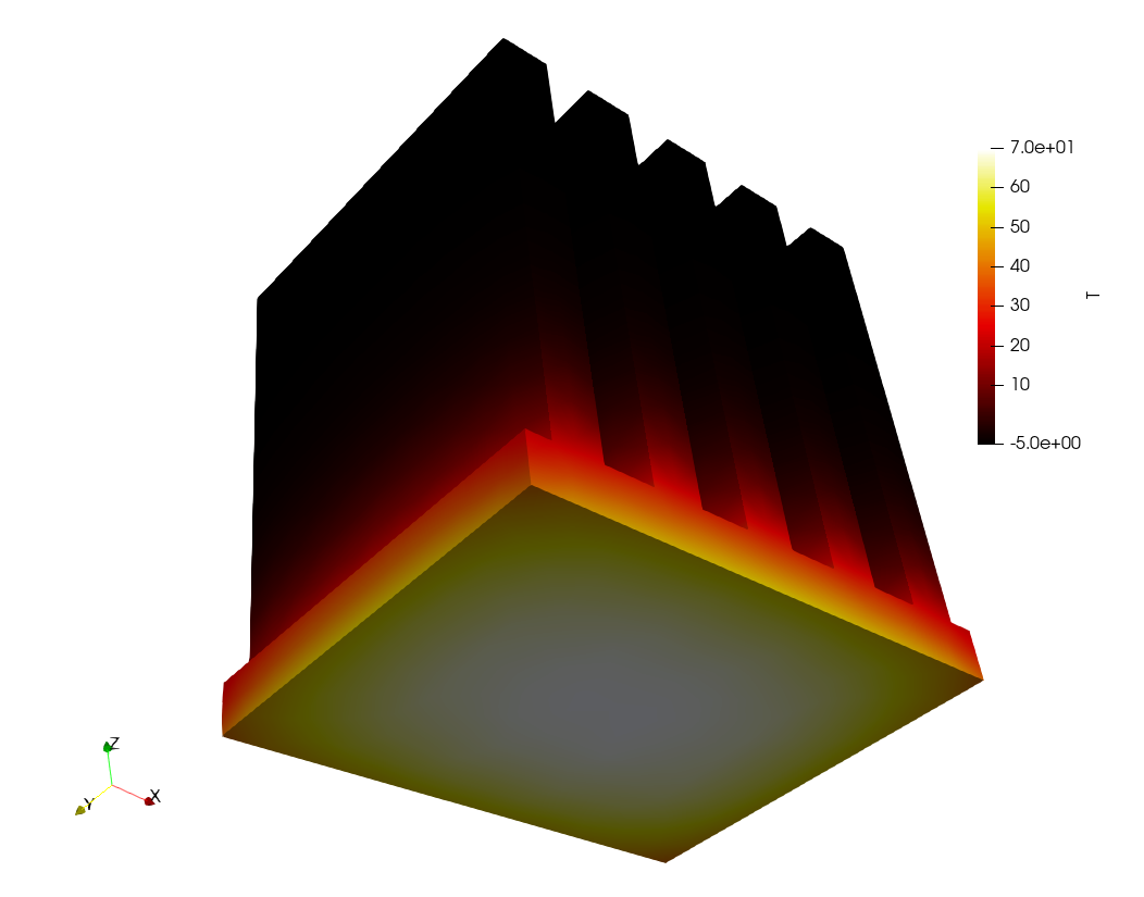
Besides being ASCII files, should special characters be needed for any reason within a particular application of FeenoX, UTF-8 characters can be used natively as illustrated in fig. 29.
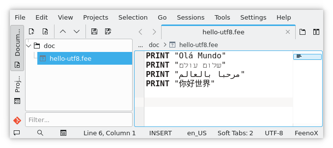
Figure 29: Special characters in Kate and in Bash.. a — UTF-8 in Kate, b — UTF-8 in Bash (through Konsole)
3.2 Results output
The output ought to contain useful results and should not be cluttered up with non-mandatory information such as ASCII art, notices, explanations or copyright notices. Since the time of cognizant engineers is far more expensive than CPU time, output should be easily interpreted by either a human or, even better, by other programs or interfaces—especially those based in mobile and/or web platforms. Open-source formats and standards should be preferred over privative and ad-hoc formatting to encourage the possibility of using different workflows and/or interfaces.
The output in FeenoX is 100% user defined, i.e. everything that FeenoX writes comes from one of the following output instructions:
In the absence of any of these instructions, FeenoX will not write anything. Not in the standard output, not in any other file. Nothing (Unix rule of silence, sec. 11.11).
| Computer | Monthly Rental | Relative Speed | First Delivery |
|---|---|---|---|
| CDC 3800 | $ 50,000 | 1 | Jan 66 |
| CDC 6600 | $ 80,000 | 6 | Sep 64 |
| CDC 6800 | $ 85,000 | 20 | Jul 67 |
| GE 635 | $ 55,000 | 1 | Nov 64 |
| IBM 360/62 | $ 58,000 | 1 | Nov 65 |
| IBM 360/70 | $ 80,000 | 2 | Nov 65 |
| IBM 360/92 | $ 142,000 | 20 | Nov 66 |
| PHILCO 213 | $ 78,000 | 2 | Sep 65 |
| UNIVAC 1108 | $ 45,000 | 2 | Aug 65 |
This is a sound design decision that follows the Unix rules of silence and, more importantly, of economy. In effect, more than fifty years ago CPU time was far more expensive than engineering time (tbl. 3). At that time, engineering programs had to write everything they computed because it was too expensive to re-run the calculation in case a single result was missing.
Nowadays the engineering time is far more expensive than CPU time. Therefore, the time needed for the user to find and process a single result in a soup of megabytes of a cluttered output file far outweighs the cost of running a computation from scratch with the needed result as the only output. Especially if the expensive engineers are smart enough to set up the problem using a coarse mesh and run the actual fine execution only after having checked everything works as expected.
The input file from the tensile-test
tutorial illustrates this idea: only 8 lines are needed to define
and solve the problem (including the instructions SOLVE_PROBLEM
and COMPUTE_REACTION)
and almost twice as much instructions for getting the required output as
needed (mostly PRINTs
and one WRITE_RESULTS):
PROBLEM mechanical MESH tensile-test.msh   # lengths are in mm

# material properties, E and nu are "special" variables for the mechanical problem
E = 200e3   # [ MPa = N / mm^2 ]
nu = 0.3

# boundary conditions, fixed and Fx are "special" keywords for the mechanical problem
# the names "left" and "right" should match the physical names in the .geo
BC left  fixed
BC right Fx=10e3  # [ N ]

# we can now solve the problem, after this keyword the results will be available for output
SOLVE_PROBLEM

# essentially we are done by now, we have to write the expected results

# 1. a VTK file to be post-processed in ParaView with
#    a. the displacements [u,v,w] as a vector
#    b. the von Mises stress sigma as a scalar
#    c. the six components of the stress tensor as six scalars
WRITE_MESH tensile-test.vtk VECTOR u v w  sigma sigmax sigmay sigmaz tauxy tauyz tauzx
PRINT "1. post-processing view written in tensile-test.vtk"

# 2. the displacement vector at the center of the specimen
PRINT "2. displacement in x at origin:   " u(0,0,0)   "[ mm ]"
PRINT "   displacement in y at (0,10,0): " v(0,10,0)  "[ mm ]"
PRINT "   displacement in z at (0,0,2.5):" w(0,0,2.5) "[ mm ]"

# 3. the principal stresses at the center
PRINT "3. principal stresses at origin: " %.4f sigma1(0,0,0) sigma2(0,0,0) sigma3(0,0,0) "[ MPa ]"

# 4. the reaction at the left surface
COMPUTE_REACTION left  RESULT R_left
PRINT "4. reaction at left surface: " R_left "[ N ]"

# 5. stress concentrations at a sharp edge
PRINT "5. stress concentrations at x=55, y=10, z=2.5 mm"
PRINT "von Mises stress:" sigma(55,10,2.5) "[ MPa ]"
PRINT "Tresca    stress:" sigma1(55,10,2.5)-sigma3(55,10,2.5) "[ MPa ]"
PRINT "stress tensor:"
PRINT %.1f sigmax(55,10,2.5) tauxy(55,10,2.5)  tauzx(55,10,2.5)
PRINT %.1f tauxy(55,10,2.5)  sigmay(55,10,2.5) tauyz(55,10,2.5)
PRINT %.1f tauzx(55,10,2.5)  tauyz(55,10,2.5)  sigmaz(55,10,2.5)
Moreover, when solving PDEs, FeenoX will be also smart enough not to
compute quantities which are not going to be written anywhere. For
example, if the input file does not reference the principal stress
sigma1 (or WRITE_RESULTS
does not ask for it) then FeenoX will not compute it.
3.2.1 Output formats
With the ASCII output to standard output (and other text files)
controlled with PRINT-like instructions, YAML or JSON
outputs can be easily implemented within the input file itself. For
example,
DEFAULT_ARGUMENT_VALUE 1 "hello world"
phi = (1+sqrt(5))/2

PRINTF "a: %.3f" 1/3
PRINT TEXT "phi:" phi SEP " "
PRINT message: ${1}   SEP " "
would give
$ feenox yaml.fee | tee test.yaml | yq .
{
  "a": 0.333,
  "phi": 1.61803,
  "message": "hello world"
}
$ cat test.yaml
a: 0.333
phi: 1.61803
message: hello world
$
Now, JSON is more picky and care with quoted characters is needed:
- Curly brackets
{and}are used for multi-line input in FeenoX so they have to be quoted as\{and\}. - Double quotes
"are used to delimit keywords with blanks, so they also have to be quoted\"when appearing verbatim in an output token.
DEFAULT_ARGUMENT_VALUE 1 "hello world"
phi = (1+sqrt(5))/2

PRINTF "\{ \"a\": %.3f," 1/3
PRINT  TEXT "\"phi\":" phi ,
PRINT  "\"message\": \"${1}\" \}"
$ feenox json.fee | jq .
{
"a": 0.333,
"phi": 1.61803,
"message": "hello world"
}
$In the same sense, in principle any ASCII-based format can be implemented this way. Markdown output, which can then be converted to other formats as well (such as LaTeX which can then create professionally-looking tables as in fig. 21), has been already covered in sec. 2.7.
Current version can write space and time-dependent distributions into
Gmsh’s .msh and VTK’s vtu/.vtk
formats. Both of them are open standard and have open-source readers.
Other formats such .med should be easy to add, but in any
case the mesh data converters such as Meshio can be used to
convert FeenoX’s post-processing output to other formats as well.
3.2.2 Data exchange between non-conformal meshes
To illustrate how the output of a FeenoX execution can be read by another FeenoX instance, let us revisit the plane-strain square from sec. 3.1.5. This time, instead of setting the temperature with an algebraic expression, we will solve a thermal problem that gives rise to the same temperature distribution but on a different mesh.
First, we solve a thermal problem on the same square [-1,+1]\times[-1,+1] such that the resulting temperature field is T(x,y) = 200 + 350\cdot y:
PROBLEM thermal 2D
READ_MESH square-centered-unstruct.msh # [-1:+1]x[-1:+1]

BC bottom    T=-150
BC top       T=+550
k = 1

SOLVE_PROBLEM
WRITE_MESH thermal-square-temperature.msh T
Now, we read the temperature T(x,y)
from the thermal output mesh file
thermal-square-temperature.msh (which is a triangular
unstructured grid) into the mechanical input mesh file
square-centered.msh (which is a structured quadrangular
grid):
PROBLEM mechanical plane_strain
READ_MESH square-centered.msh # [-1:+1]x[-1:+1]

# fixed at left, uniform traction in the x direction at right
BC left    fixed
BC right   tx=50

# ASME II Part D pag. 785 Carbon steels with C<=0.30%
FUNCTION E_carbon(temp) INTERPOLATION steffen DATA {
-200  216
-125  212
-75   209
25    202
100   198
150   195
200   192
250   189
300   185
350   179
400   171
450   162
500   151
550   137
}

# read the temperature from a previous result
READ_MESH thermal-square-temperature.msh DIM 2 READ_FUNCTION T

# Young modulus is the function above evaluated at the local temperature
E(x,y) := E_carbon(T(x,y))

# uniform Poisson's ratio
nu = 0.3

SOLVE_PROBLEM
WRITE_MESH mechanical-square-temperature-from-msh.vtk  E T VECTOR u v 0
Indeed, the terminal mimic shows the difference between the mechanical input from this section and the one that used an explicit algebraic expression.
$ gmsh -2 square-centered-unstruct.geo
[...]
Info    : Done meshing 2D (Wall 0.012013s, CPU 0.033112s)
Info    : 65 nodes 132 elements
Info    : Writing 'square-centered-unstruct.msh'...
Info    : Done writing 'square-centered-unstruct.msh'
Info    : Stopped on Wed Aug  3 17:47:39 2022 (From start: Wall 0.0208329s, CPU 0.064825s)
$ feenox thermal-square.fee
$ feenox mechanical-square-temperature-from-msh.fee
$ diff mechanical-square-temperature-from-msh.fee mechanical-square-temperature.fee
26,27c26,29
< # read the temperature from a previous result
< READ_MESH thermal-square-temperature.msh DIM 2 READ_FUNCTION T
---
>
> # known temperature distribution
> # (we could have read it from an output of a thermal problem)
> T(x,y) := 200 + 350*y
36c38
< WRITE_MESH mechanical-square-temperature-from-msh.vtk  E T VECTOR u v 0
---
> WRITE_MESH mechanical-square-temperature.vtk  E  VECTOR u v 0
$
4 Quality assurance
Since the results obtained with the tool might be used in verifying existing equipment or in designing new mechanical parts in sensitive industries, a certain level of software quality assurance is needed. Not only are best-practices for developing generic software such as
- employment of a version control system,
- automated testing suites,
- user-reported bug tracking support.
- etc.
required, but also since the tool falls in the category of engineering computational software, verification and validation procedures are also mandatory, as discussed below. Design should be such that governance of engineering data including problem definition, results and documentation can be efficiently performed using state-of-the-art methodologies, such as distributed control version systems
The development of FeenoX is tracked with the distributed version control system Git. The official repository is hosted on Github at https://github.com/seamplex/feenox/. New non-trivial features are added in new branches which are then eventually merged into the main branch.
Note that nowadays mentioning that the source code of a piece of software is tracked with Git (why wouldn’t it?) is like saying a hotel has a private bathroom in each room (why wouldn’t it?). But the reader ought to keep in mind that there is a non-negligible fraction of production calculation codes (even nuclear-related) whose source code is not tracked with a DVCS, let alone features and bug fixes follow the branch-review-merge path.
4.1 Reproducibility and traceability
The full source code and the documentation of the tool ought to be maintained under a control version system. Whether access to the repository is public or not is up to the vendor, as long as the copying conditions are compatible with the definitions of both free and open source software from the FSF and the OSI, respectively as required in sec. 1.
In order to be able to track results obtained with different version of the tools, there should be a clear release procedure. There should be periodical releases of stable versions that are required
- not to raise any warnings when compiled using modern versions of common compilers (e.g. GNU, Clang, Intel, etc.)
- not to raise any errors when assessed with dynamic memory analysis tools (e.g. Valgrind) for a wide variety of test cases
- to pass all the automated test suites as specified in sec. 4.2
These stable releases should follow a common versioning scheme, and either the tarballs with the sources and/or the version control system commits should be digitally signed by a cognizant responsible. Other unstable versions with partial and/or limited features might be released either in the form of tarballs or made available in a code repository. The requirement is that unstable tarballs and main (a.k.a. trunk) branches on the repositories have to be compilable. Any feature that does not work as expected or that does not even compile has to be committed into develop branches before being merge into trunk.
If the tool has an executable binary, it should be able to report which version of the code the executable corresponds to. If there is a library callable through an API, there should be a call which returns the version of the code the library corresponds to.
It is recommended not to mix mesh data like nodes and element definition with problem data like material properties and boundary conditions so as to ease governance and tracking of computational models and the results associated with them. All the information needed to solve a particular problem (i.e. meshes, boundary conditions, spatially-distributed material properties, etc.) should be generated from a very simple set of files which ought to be susceptible of being tracked with current state-of-the-art version control systems. In order to comply with this suggestion, ASCII formats should be favored when possible.
As stated in the previous section, the official repository is freely available on Github. As long as the copying conditions (GPLv3+) are met, the repository can be freely cloned and/or forked.
Each binary executable feenox has embedded a literal
string with the version of the source code used to build it. When
running without arguments, it will print the version (which includes the
hash of the last commit to the repository) and the usage:
$ feenox
FeenoX v1.0.7-g9b98430
a cloud-first free no-fee no-X uniX-like finite-element(ish) computational engineering tool

usage: feenox [options] inputfile [replacement arguments] [petsc options]

  -h, --help         display options and detailed explanations of command-line usage
  -v, --version      display brief version information and exit
  -V, --versions     display detailed version information
  -c, --check        validates if the input file is sane or not
  --pdes             list the types of PROBLEMs that FeenoX can solve, one per line
  --elements_info    output a document with information about the supported element types
  --linear           force FeenoX to solve the PDE problem as linear
  --non-linear       force FeenoX to solve the PDE problem as non-linear

Run with --help for further explanations.
$
As required by the GNU Standards, running with -v or
--version will print copyright information as well:
$ feenox -v
FeenoX v1.0.7-g9b98430
a cloud-first free no-fee no-X uniX-like finite-element(ish) computational engineering tool

Copyright © 2009--2024 https://seamplex.com/feenox
GNU General Public License v3+, https://www.gnu.org/licenses/gpl.html.
FeenoX is free software: you are free to change and redistribute it.
There is NO WARRANTY, to the extent permitted by law.
$
And running with -V or --versions will
print detailed versioning information about
- the date and time of the last commit to the repository
- the date and time of compilation
- the architecture, compiler type, version and flags used to build the executable
- the versions of the external numerical libraries used to link the executable
$ feenox --versions
FeenoX v1.0.7-g9b98430
a cloud-first free no-fee no-X uniX-like finite-element(ish) computational engineering tool

Last commit date   : Tue Mar 19 16:17:30 2024 -0300
Build date         : Wed Mar 20 07:40:34 2024 -0300
Build architecture : linux-gnu x86_64
Compiler version   : gcc (Debian 12.2.0-14) 12.2.0
Compiler expansion : gcc -Wl,-z,relro -I/usr/include/x86_64-linux-gnu/mpich -L/usr/lib/x86_64-linux-gnu -lmpich
Compiler flags     : -O3 -flto=auto -no-pie
Builder            : gtheler@tom
GSL version        : 2.7.1
SUNDIALS version   : N/A
PETSc version      : Petsc Development GIT revision: v3.20.5-856-g0d3f65ad054  GIT Date: 2024-03-20 02:13:21 +0000
PETSc arch         : arch-linux-c-debug
PETSc options      : --download-eigen --download-hdf5 --download-hypre --download-metis --download-mumps --download-parmetis --download-scalapack --download-slepc --with-64-bit-indices=no --with-debugging=yes --with-precision=double --with-scalar-type=real PETSC_ARCH=arch-linux-c-debug --force
SLEPc version      : SLEPc Development GIT revision: v3.20.1-36-g7a35a7b97  GIT Date: 2023-12-02 02:30:03 -0600
$
The version is composed of three dot-separated integers:
- the major version (major changes)
- the minor version (incompatible input changes)
- the revision (individual commits from last tag)
The autogen.sh script builds this string at compile
time, which is stored in a header and finally embedded into the
executable. The major m and minor n integers are read from the git tag
formatted as vm.n, which is bumped manually by adding an
annotated tag to a particular commit. The revision is computed
automatically with git describe as the number of commits in
the main branch from the tag to the last commit. The hash is also added
to avoid ambiguities in case the repository is forked and diverged from
the official one. Periodically, source and binary tarballs are built
(using automated scripts in the dist subdirectory) and
published online.
Given the input-file scheme thoroughfully explained in
sec. 3.1—especially the separation of the problem formulation from the
mesh data–the input files can be tracked with Git (or any other VCS) as
well, therefore enhancing traceability of results and data governance.
Again, this might be obvious in the 2020s. But there are many FEM
solvers which mix the mesh data with the problem definition (e.g. when
external loads have to be given at the nodes instead of using
expressions like p=rho*g*z or Fx=1e3).
4.2 Automated testing
A mean to automatically test the code works as expected is mandatory. A set of problems with known solutions should be solved with the tool after each modification of the code to make sure these changes still give the right answers for the right questions and no regressions are introduced. Unit software testing practices like continuous integration and test coverage are recommended but not mandatory.
The tests contained in the test suite should be
- varied,
- diverse, and
- independent
Due to efficiency issues, there can be different sets of tests (e.g. unit and integration tests, quick and thorough tests, etc.) Development versions stored in non-main branches can have temporarily-failing tests, but stable versions have to pass all the test suites.
The make check target will execute a set of Bash scripts
which will run hundreds of cases and compare their solutions to
reference values. These references might be
- analytical solutions,
- known reference solutions, or
- random reference solutions.
Depending on the type of case being run, some of these tests might work as very simplified verification cases. But the bulk work as regressions tests so developers adding new features can check they do not break existing working code.
For example, if by mistake a developer flips a sign of one term when setting convection boundary conditions in the heat-conduction PDE, i.e. from
double rhs = h*Tref;to
double rhs = -h*Tref;then the make check step will detect it. In effect,
$ make check
[...]
XFAIL: tests/abort.sh
PASS: tests/algebraic_expr.sh
PASS: tests/annulus-modal.sh
PASS: tests/uo2-pellet.sh
[...]
PASS: tests/t21.sh
FAIL: tests/thermal-1d.sh
PASS: tests/thermal-2d.sh
FAIL: tests/thermal-3d.sh
XFAIL: tests/thermal-slab-no-k.sh
XFAIL: tests/thermal-slab-wrong-bc.sh
FAIL: tests/thermal-radiation.sh
PASS: tests/transient-mesh.sh
PASS: tests/trig.sh
[...]
============================================================================
Testsuite summary for feenox 1.0.7
============================================================================
# TOTAL: 75
# PASS:  64
# SKIP:  2
# XFAIL: 6
# FAIL:  3
# XPASS: 0
# ERROR: 0
============================================================================
See ./test-suite.log
Please report to jeremy@seamplex.com
============================================================================
make[3]: *** [Makefile:1723: test-suite.log] Error 1
[...]
make: *** [Makefile:1608: check-recursive] Error 1
$
4.3 Bug reporting and tracking
A system to allow developers and users to report bugs and errors and to suggest improvements should be provided. If applicable, bug reports should be tracked, addressed and documented. User-provided suggestions might go into the back log or TO-DO list if appropriate.
Here, “bug and errors” mean failure to
- compile on supported architectures,
- run (unexpected run-time errors, segmentation faults, etc.)
- return a correct result
The Github Issues feature at https://github.com/seamplex/feenox/issues is used to report and track bugs and errors (fig. 30).
4.4 Documentation
Documentation should be complete and cover both the user and the developer point of view. It should include a user manual adequate for both reference and tutorial purposes. Other forms of simplified documentation such as quick reference cards or video tutorials are not mandatory but highly recommended. Since the tool should be extendable (sec. 2.6), there should be a separate development manual covering the programming design and implementation, explaining how to extend the code and how to add new features. Also, as non-trivial mathematics which should be verified are expected, a thorough explanation of what equations are taken into account and how they are solved is required.
It should be possible to make the full documentation available online in a way that it can be both printed in hard copy and accessed easily from a mobile device. Users modifying the tool to suit their own needs should be able to modify the associated documentation as well, so a clear notice about the licensing terms of the documentation itself (which might be different from the licensing terms of the source code itself) is mandatory. Tracking changes in the documentation should be similar to tracking changes in the code base. Each individual document ought to explicitly state to which version of the tool applies. Plain ASCII formats should be preferred. It is forbidden to submit documentation in a non-free format.
The documentation shall also include procedures for
- reporting errors and bugs
- releasing stable versions
- performing verification and validation studies
- contributing to the code base, including
- code of conduct
- coding styles
- variable and function naming conventions
According to Eric Raymond’s book “The Art of Unix Programming”:
Compactness is the property that a design can fit inside a human being’s head. A good practical test for compactness is this: Does an experienced user normally need a manual? If not, then the design (or at least the subset of it that covers normal use) is compact.
Following to 20-80 rule, we could say that FeenoX is compact for 80%
of its usage. But the most complex 20% of the cases might need users
(even the author) to look up the syntax of the definition and
instructions in the manual page (illustrated in fig. 31), which is
accessible with man feenox after installing with
make install:
$ man -k feenox
feenox (1)           - a cloud-first free no-X uniX-like finite-element(ish) computational engineering tool
$ man feenox
$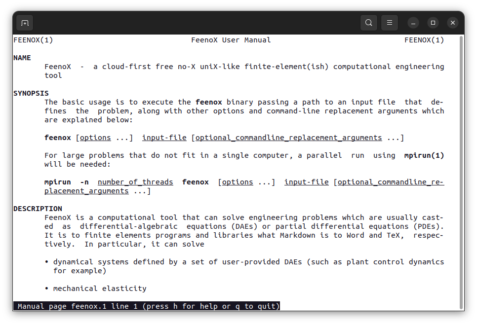
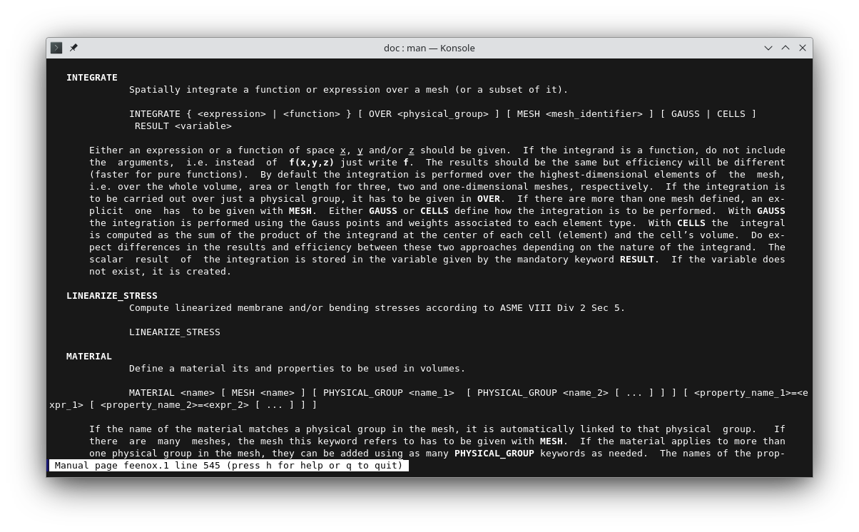
Figure 31: The FeenoX Unix manpage in section 1 when
running man feenox. a — Gnome Terminal, b —
Konsole
This man page is compiled into troff from a markdown source, which in turn has some sections involving the syntax and reference of the
- definitions and instructions
- special variables
- internal built-in functions and functionals
generated by a script that parses the actual source code. For
instance, the code that parses the INTEGRATE function has
three-forward-slash comments that tell this script that it has to
prepare documentation:
int feenox_parse_integrate(void) {

  mesh_integrate_t *mesh_integrate = NULL;
  feenox_check_alloc(mesh_integrate = calloc(1, sizeof(mesh_integrate_t)));

///kw_pde+INTEGRATE+usage { <expression> | <function> }
///kw_pde+INTEGRATE+detail Either an expression or a function of space $x$, $y$ and/or $z$ should be given.
///kw_pde+INTEGRATE+detail If the integrand is a function, do not include the arguments, i.e. instead of `f(x,y,z)` just write `f`.
///kw_pde+INTEGRATE+detail The results should be the same but efficiency will be different (faster for pure functions).
  char *token = feenox_get_next_token(NULL);
  if ((mesh_integrate->function = feenox_get_function_ptr(token)) == NULL) {
    feenox_call(feenox_expression_parse(&mesh_integrate->expr, token));
  }

  char *name_mesh = NULL;
  char *name_physical_group = NULL;
  char *name_result = NULL;

  while ((token = feenox_get_next_token(NULL)) != NULL) {
///kw_pde+INTEGRATE+usage [ OVER <physical_group> ]
///kw_pde+INTEGRATE+detail By default the integration is performed over the highest-dimensional elements of the mesh,
///kw_pde+INTEGRATE+detail i.e. over the whole volume, area or length for three, two and one-dimensional meshes, respectively.
///kw_pde+INTEGRATE+detail If the integration is to be carried out over just a physical group, it has to be given in `OVER`.

    if (strcasecmp(token, "OVER") == 0) {
      feenox_call(feenox_parser_string(&name_physical_group));

[...]
The script doc/reference.sh would create the markdown
snippet shown in fig. 32 (a), which then can be converted to other
output formats (figs. 32 (b), 32 (c), 32 (d)) for the final user (and
author) to look up the syntax of the input keywords.
Figure 32: Reference for the keyword
INTEGRATE in Markdown created out of special comments in
the C source converted to different output formats.. a — Markdown, b —
Manpage, c — HTML, d — PDF
Other pieces of documentation in markdown which then are converted to HTML & PDF (with Pandoc and XeLaTeX) include:
- The FeenoX manual
- The FeenoX description (converted to Texinfo as well)
- Software Requirements Specification
- Software Design Specification
- Frequently Asked Questions
- FeenoX Unix man page
- History
- Compilation guide
- Programming guide
5 Appendix: Downloading and compiling FeenoX
5.1 Debian & Ubuntu packages
To be explained
5.2 Binary executables
Browse to https://www.seamplex.com/feenox/dist/ and check what the latest version for your architecture is. Then do
feenox_version=1.1
wget -c https://www.seamplex.com/feenox/dist/linux/feenox-v${feenox_version}-linux-amd64.tar.gz
tar xzf feenox-v${feenox_version}-linux-amd64.tar.gz
sudo cp feenox-v${feenox_version}-linux-amd64/bin/feenox /usr/local/bin
You’ll have the binary under bin and examples,
documentation, manpage, etc under share. Copy
bin/feenox into somewhere in the PATH and that
will be it. If you are root, do
sudo cp feenox-v${feenox_version}-linux-amd64/bin/feenox /usr/local/binIf you are not root, the usual way is to create a directory
$HOME/bin and add it to your local path. If you have not
done it already, do
mkdir -p $HOME/bin
echo 'expot PATH=$PATH:$HOME/bin' >> .bashrc
Then finally copy bin/feenox to
$HOME/bin
cp feenox-v${feenox_version}-linux-amd64/bin/feenox $HOME/binCheck if it works by calling feenox from any directory
(you might need to open a new terminal so .bashrc is
re-read):
$ feenox
FeenoX v1.1-g94ddf72
a cloud-first free no-fee no-X uniX-like finite-element(ish) computational engineering tool

usage: feenox [options] inputfile [replacement arguments] [petsc options]

  -h, --help         display options and detailed explanations of command-line usage
  -v, --version      display brief version information and exit
  -V, --versions     display detailed version information
  -c, --check        validates if the input file is sane or not
  --pdes             list the types of PROBLEMs that FeenoX can solve, one per line
  --elements_info    output a document with information about the supported element types
  --ast              dump an abstract syntax tree of the input
  --linear           force FeenoX to solve the PDE problem as linear
  --non-linear       force FeenoX to solve the PDE problem as non-linear

Run with --help for further explanations.
$
5.3 Source tarballs
To compile the source tarball, proceed as follows. This procedure
does not need git nor autoconf but a new source tarball has to be downloaded each time there is a new
FeenoX version.
Install mandatory dependencies
sudo apt-get update
sudo apt-get install gcc make libgsl-dev
If you cannot install
libgsl-dev, you can have theconfigurescript to download and compile it for you. See point 4 below.Install optional dependencies (of course these are optional but recommended)
sudo apt-get install libsundials-dev petsc-dev slepc-devDownload and un-compress FeenoX source tarball. Browse to https://www.seamplex.com/feenox/dist/src/ and pick the latest version:
wget https://www.seamplex.com/feenox/dist/src/feenox-v1.1.tar.gz
tar xvzf feenox-v1.1.tar.gz
Configure, compile & make
cd feenox-v1.1
./configure
make -j4
If you cannot (or do not want) to use
libgsl-devfrom a package repository, callconfigurewith--enable-download-gsl:./configure --enable-download-gslIf you do not have Internet access, get the tarball manually, copy it to the same directory as
configureand run again.Run test suite (optional)
make checkInstall the binary system wide (optional)
sudo make install
5.4 Git repository
The Git repository has the latest sources repository. To compile, proceed as follows. If something goes wrong and you get an error, do not hesitate to ask in FeenoX’s discussion page.
If you do not have Git or Autotools, download a source tarball and proceed with the usual
configure&makeprocedure. See these instructions.
Install mandatory dependencies
sudo apt-get update
sudo apt-get install git build-essential make automake autoconf libgsl-dev
If you cannot install
libgsl-devbut still havegitand the build toolchain, you can have theconfigurescript to download and compile it for you. See point 4 below.Install optional dependencies (of course these are optional but recommended)
sudo apt-get install libsundials-dev petsc-dev slepc-devClone Github repository
git clone https://github.com/seamplex/feenoxBootstrap, configure, compile & make
cd feenox
./autogen.sh
./configure
make -j4
If you cannot (or do not want to) use
libgsl-devfrom a package repository, callconfigurewith--enable-download-gsl:./configure --enable-download-gslIf you do not have Internet access, get the tarball manually, copy it to the same directory as
configureand run again. See the detailed compilation instructions for an explanation.Run test suite (optional)
make checkInstall the binary system wide (optional)
sudo make installIf you do not have root permissions, configure with your home directory as prefix and then make install as a regular user:
./configure --prefix=$HOME
make
make install
export PATH=$PATH:$HOME/bin
To stay up to date, pull and then autogen,
configure and make (and optionally
install):
git pull
./autogen.sh
./configure
make -j4
sudo make install
6 Appendix: Rules of Unix philosophy
In 1978, Doug McIlroy—the inventor of Unix pipes and one of the founders of the Unix tradition—stated:
Make each program do one thing well. To do a new job, build afresh rather than complicate old programs by adding new features.
Expect the output of every program to become the input to another, as yet unknown, program. Don’t clutter output with extraneous information. Avoid stringently columnar or binary input formats. Don’t insist on interactive input.
Design and build software, even operating systems, to be tried early, ideally within weeks. Don’t hesitate to throw away the clumsy parts and rebuild them.
Use tools in preference to unskilled help to lighten a programming task, even if you have to detour to build the tools and expect to throw some of them out after you’ve finished using them.
He later summarized it this way:
This is the Unix philosophy: Write programs that do one thing and do it well. Write programs to work together. Write programs to handle text streams, because that is a universal interface.
FeenoX explicitly followed the above ideas from scratch, especially the for sentences in bullet ii. It is even, like Unix itself, a third-system effect where clumsy parts of previous attempts were thrown away and rebuilt from scratch. The following sections explain how each of the seventeen rules was taken into account when designing and implementing FeenoX.
6.1 Rule of Modularity
Developers should build a program out of simple parts connected by well defined interfaces, so problems are local, and parts of the program can be replaced in future versions to support new features. This rule aims to save time on debugging code that is complex, long, and unreadable.
FeenoX is designed to be as lightweight as possible. On the one hand, it relies on third-party high-quality libraries to do the heavy mathematical weightlifting such as
- GNU Scientific Library for general mathematics,
- SUNDIALS IDA for ODEs and DAEs,
- PETSc for linear, non-linear and transient PDEs, and
- SLEPc for PDEs involving eigen problems
because these libraries were written by professional programmers using algorithms designed by professional mathematicians. Yet-to-be-discovered improved mathematical schemes and/or coding algorithms can be eventually used by FeenoX by just updating those dependencies, which for sure will keep their well-defined interfaces (because they are programmed by professional programmers).
Moreover, the extensibility feature (sec. 11.17) of having each PDE in separate directories which can be added or removed at compile time without changing any line of the source code goes into this direction as well. Relying of C function pointers allows (in principle) to replace these “virtual” methods with other ones using the same interface.
Note that our (human) languages in general and words in particular shape and limit the way we think. Fortran’s concept of “modules” is not the same as Unix’s concept of “modularity.” I wish two different words had been used.
6.2 Rule of Clarity
Developers should write programs as if the most important communication is to the developer who will read and maintain the program, rather than the computer. This rule aims to make code as readable and comprehensible as possible for whoever works on the code in the future.
Of course there might be a confirmation bias in this section because every programmer thinks their code is clear (and everybody else’s is not). But the first design decision to fulfill this rule is the programming language: there is little change to fulfill it with Fortran. One might argue that C++ can be clearer than C in some points, but for the vast majority of the source code they are equally clear. Besides, C is far simpler than C++ (see rule of simplicity).
The second decision is not about the FeenoX source code but about FeenoX inputs: clear human-readable input files without any extra unneeded computer-level nonsense. The two illustrative cases are the NAFEMS LE10 & LE11 benchmarks, where there is a clear one-to-one correspondence between the “engineering” formulation and the input file FeenoX understands.
6.3 Rule of Composition
Developers should write programs that can communicate easily with other programs. This rule aims to allow developers to break down projects into small, simple programs rather than overly complex monolithic programs.
Previous designs of FeenoX’ predecessors used to include instructions
to perform parametric sweeps( and even optimization loops), non-trivial
macro expansions using M4 and even execution of arbitrary shell
commands. These non-trivial operations were removed from FeenoX to focus
on the rule of composition, paying especially attention to easing the
inclusion of calling the feenox binary from shell scripts,
enforcing the composition with other Unix-like tools. Emphasis has been
put on adding flexibility to programmatic generation of input files (see
also rule of generation in sec. 11.14) and the handling and expansion of
command-line arguments to increase the composition with other
programs.
Moreover, the output is 100% controlled by the user at run-time so it can be tailored to suit any other programs’ input needs as well. An illustrative example is creating professional-looking tables with results using AWK & LaTeX.
6.4 Rule of Separation
Developers should separate the mechanisms of the programs from the policies of the programs; one method is to divide a program into a front-end interface and a back-end engine with which that interface communicates. This rule aims to prevent bug introduction by allowing policies to be changed with minimum likelihood of destabilizing operational mechanisms.
FeenoX relies of the rule of separation (which also links to the next two rules of simplicity and parsimony) from the very beginning of its design phase. It was explicitly designed as a glue layer between a mesher like Gmsh and a post-processor like Gnuplot, Gmsh or Paraview. This way, not only flexibility and diversity (see #sec:unix-diversity) can be boosted, but also technological changes can be embraced with little or no effort. For example, CAEplex provides a web-based platform for performing thermo-mechanical analysis on the cloud running from the browser. Had FeenoX been designed as a traditional desktop-GUI program, this would have been impossible. If in the future CAD/CAE interfaces migrate into virtual and/or augmented reality with interactive 3D holographic input/output devices, the development effort needed to use FeenoX as the back end is negligible.
6.5 Rule of Simplicity
Developers should design for simplicity by looking for ways to break up program systems into small, straightforward cooperating pieces. This rule aims to discourage developers’ affection for writing “intricate and beautiful complexities” that are in reality bug prone programs.
The main source of simplicity comes from the design of the syntax of the input files, discussed in detail in the SDS:
- English-like self-evident input files matching as close as possible the problem text.
- Simple problems need simple input.
- Similar problems need similar inputs.
- If there is a single material there is no need to link volumes to properties.
6.6 Rule of Parsimony
Developers should avoid writing big programs. This rule aims to prevent overinvestment of development time in failed or suboptimal approaches caused by the owners of the program’s reluctance to throw away visibly large pieces of work. Smaller programs are not only easier to write, optimize, and maintain; they are easier to delete when deprecated.
We already said that FeenoX is a glue layer between a mesher and a post-processing tool. Even more, at another level, it acts as two glue layers between the mesher and PETSc, and PETSc and the post-processor.
On the other hand, we also already stated that FeenoX was written from scratch after throwing away clumsy code from two previous attempts. For instance, these previous versions used to implement parametric and optimization schemes. Instead, in FeenoX, these type of runs have to be driven from an outer script (Bash, Python, etc.)
6.7 Rule of Transparency
Developers should design for visibility and discoverability by writing in a way that their thought process can lucidly be seen by future developers working on the project and using input and output formats that make it easy to identify valid input and correct output. This rule aims to reduce debugging time and extend the lifespan of programs.
As with the rule of clarity (sec. 11.2), there is a risk of falling into the confirmation bias because every programmer thinks its code is transparent. Anyway, FeenoX is written in C99 which is way easier to debug than both Fortran and C++. Yet, very much like PETSc, FeenoX makes use of structures and function pointers to give the same functionality as C++’s virtual methods without needing to introduce other complexities that make the code base harder to maintain and to debug.
Regarding identification of valid inputs and correct outputs,
- The build system includes a
make checktarget that runs hundreds of regressions tests. - The code supports verification using the Method of Manufactured Solutions
6.8 Rule of Robustness
Developers should design robust programs by designing for transparency and discoverability, because code that is easy to understand is easier to stress test for unexpected conditions that may not be foreseeable in complex programs. This rule aims to help developers build robust, reliable products.
Robustness is the child of transparency and simplicity.
6.9 Rule of Representation
Developers should choose to make data more complicated rather than the procedural logic of the program when faced with the choice, because it is easier for humans to understand complex data compared with complex logic. This rule aims to make programs more readable for any developer working on the project, which allows the program to be maintained.
There is a trade off between clarity and efficiency. However,
avoiding Fortran should already fulfill this rule. FeenoX uses C
structures with function pointers, which make it far simple to
understand than similar Fortran-based FEM tools. Just compare the source
directories of FeenoX and CalculiX. Take for instance the file stress.c
from src/pdes/mechanical
(which if deleted, will remove support for mechanical
problems but it will not prevent the compilation of feenox)
from the former and calcstress.f
(buried inside 2,400 files in src)
from the latter. There might be more illustrative examples showing how
FeenoX’ design is more representative than of CalculiX, but it is way
too hard to understand the source code of the latter (even though the
license is supposed to be GPL).
6.10 Rule of Least Surprise
Developers should design programs that build on top of the potential users’ expected knowledge; for example, ‘+’ in a calculator program should always mean ‘addition’. This rule aims to encourage developers to build intuitive products that are easy to use.
The rules of input syntax have been designed with this rule in mind. Just note a couple of them:
The command-line arguments after the input file are available to be expanded verbatim in the input file as
$1,$2, etc. (or${1},${2}, etc. if they appear in the middle of strings). This syntax matches Bash’ syntax for expanding command-line arguments, so any person reading an input file with this syntax already knows what it does. ´If one needs a problem where the conductivity depends on x as k(x)=1+x then the input is
k(x) = 1+xIf a problem needs a temperature distribution given by an algebraic expression T(x,y,z)=\sqrt{x^2+y^2}+z then do
T(x,y,z) = sqrt(x^2+y^2) + zThis syntax for (basic) algebraic expressions matches the common syntax found in Gmsh, Maxima and many other scientific tools. More complex expressions (e.g. involving hyperbolic tangents) might differ slightly.
6.11 Rule of Silence
Developers should design programs so that they do not print unnecessary output. This rule aims to allow other programs and developers to pick out the information they need from a program’s output without having to parse verbosity.
TL;DR: no PRINT (or WRITE_RESULTS), no
output.
6.12 Rule of Repair
Developers should design programs that fail in a manner that is easy to localize and diagnose or in other words “fail noisily”. This rule aims to prevent incorrect output from a program from becoming an input and corrupting the output of other code undetected.
Input errors are detected before the computation is started:
$ feenox thermal-error.fee
error: undefined thermal conductivity 'k'
$
Run-time errors (even inside the numerical libraries) are caught with custom handlers.
6.13 Rule of Economy
Developers should value developer time over machine time, because machine cycles today are relatively inexpensive compared to prices in the 1970s. This rule aims to reduce development costs of projects.
As explained in the SDS, output is 100% user-defined so only the desired results are directly obtained instead of needing further digging into tons of undesired data. The approach of “compute and write everything you can in one single run” made sense in 1970 where CPU time was more expensive than human time, but not anymore. Once again, the iconic examples are the NAFEMS LE10 & LE11 benchmarks, where just the required scalar stress at the required location is written into the standard output.
6.14 Rule of Generation
Developers should avoid writing code by hand and instead write abstract high-level programs that generate code. This rule aims to reduce human errors and save time.
Some key points:
- Input files are M4-like-macro friendly.
- Parametric runs can be done from scripts through expansion of command line arguments.
- Documentation is created out of simple Markdown sources and assembled as needed.
More saliently, the automatic detection of the available PDEs in
src/pdes is an example of this rule. The
autogen.sh would loop over each subdirectory and create a
source file src/pdes/parser.c with a function
feenox_pde_parse_problem_type() which then will be part of
the actual FeenoX source base as the entry point for parsing the
PROBLEM keyword.
6.15 Rule of Optimization
Developers should prototype software before polishing it. This rule aims to prevent developers from spending too much time for marginal gains.
FeenoX is still “premature” for heavy optimization. Yet, it is (relatively) faster than other alternatives. It does use link-time optimization to allow for inlining of small routines. There is even a FeenoX benchmarking repository that uses Google’s Benchmark library to prototype code optimization: https://github.com/seamplex/feenox-benchmark.
6.16 Rule of Diversity
Developers should design their programs to be flexible and open. This rule aims to make programs flexible, allowing them to be used in ways other than those their developers intended.
FeenoX can read Gmsh files, but they need not necessarily be created by Gmsh. Other meshing formats (VTK with group names?) are planned to be implemented. Also, either Gmsh or Paraview can be used to post-process results. But also other formats are planned. See sec. 11.17. Diversity is embraced from the bottom up!
6.17 Rule of Extensibility
Developers should design for the future by making their protocols extensible, allowing for easy plugins without modification to the program’s architecture by other developers, noting the version of the program, and more. This rule aims to extend the lifespan and enhance the utility of the code the developer writes.
The main extensibility feature is that each PDE has a separate source directory. Any of them can be used as as template to add new PDEs, which are detected at compile time by the Autotools bootstrapping script.
A final note is that FeenoX is GPLv3+. First, this means that
extensions and contributions are welcome. Each author retains the
copyright on the contributed code (as long as it is free software).
Second, the + is there for the future.
7 Appendix: FeenoX history
Very much like Unix in the late 1960s and C in the early 1970s, FeenoX is a third-system effect: I wrote a first hack that seemed to work better than I had expected. Then I tried to add a lot of features and complexities which I felt the code needed. After ten years of actual usage, I then realized
- what was worth keeping,
- what needed to be rewritten and
- what had to be discarded.
The first version was called wasora, the second was “The wasora suite” (i.e. a generic framework plus a bunch of “plugins”, including a thermo-mechanical one named Fino) and then finally FeenoX. The story that follows explains why I wrote the first hack to begin with.
It was at the movies when I first heard about dynamical systems, non-linear equations and chaos theory. The year was 1993, I was ten years old and the movie was Jurassic Park. Dr. Ian Malcolm (the character portrayed by Jeff Goldblum) explained sensitivity to initial conditions in a memorable scene, which is worth watching again and again. Since then, the fact that tiny variations may lead to unexpected results has always fascinated me. During high school I attended a very interesting course on fractals and chaos that made me think further about complexity and its mathematical description. Nevertheless, it was not not until college that I was able to really model and solve the differential equations that give rise to chaotic behavior.

In fact, initial-value ordinary differential equations arise in a great variety of subjects in science and engineering. Classical mechanics, chemical kinetics, structural dynamics, heat transfer analysis and dynamical systems, among other disciplines, heavily rely on equations of the form
\dot{\mathbf{x}} = F(\mathbf{x},t)
During my years of undergraduate student (circa 2004–2007), whenever I had to solve these kind of equations I had to choose one of the following three options:
- to program an ad-hoc numerical method such as Euler or Runge-Kutta, matching the requirements of the system of equations to solve, or
- to use a standard numerical library such as the GNU Scientific Library and code the equations to solve into a C program (or maybe in Python), or
- to use a high-level system such as Octave, Maxima, or some non-free (and worse, see below) programs.
Of course, each option had its pros and its cons. But none provided the combination of advantages I was looking for, namely flexibility (option one), efficiency (option two) and reduced input work (partially given by option three). Back in those days I ended up wandering between options one and two, depending on the type of problem I had to solve. However, even though one can, with some effort, make the code read some parameters from a text file, any other drastic change usually requires a modification in the source code—some times involving a substantial amount of work—and a further recompilation of the code. This was what I most disliked about this way of working, but I could nevertheless live with it.
Regardless of this situation, during my last year of Nuclear Engineering, the tipping point came along. Here’s a slightly-fictionalized of a dialog between myself and the teacher at the computer lab (Dr E.), as it might have happened (or not):
— (Prof.) Open MATLAB.™
— (Me) It’s not installed here. I typemathlaband it does not work.
— (Prof.) It’s spelledmatlab.
— (Me) Ok, working. (A screen with blocks and lines connecting them appears)
— (Me) What’s this?
— (Prof.) The point reactor equations.
— (Me) It’s not. These are the point reactor equations:\begin{cases} \dot{\phi}(t) = \displaystyle \frac{\rho(t) - \beta}{\Lambda} \cdot \phi(t) + \sum_{i=1}^{N} \lambda_i \cdot c_i \\ \dot{c}_i(t) = \displaystyle \frac{\beta_i}{\Lambda} \cdot \phi(t) - \lambda_i \cdot c_i \end{cases}
— (Me) And in any case, I’d write them like this in a computer:
phi_dot = (rho-Beta)/Lambda * phi + sum(lambda[i], c[i], i, 1, N)
c_dot[i] = beta[i]/Lambda * phi - lambda[i]*c[i]
This conversation forced me to re-think the ODE-solving issue. I could not (and still cannot) understand why somebody would prefer to solve a very simple set of differential equations by drawing blocks and connecting them with a mouse with no mathematical sense whatsoever. Fast forward fifteen years, and what I wrote above is essentially how one would solve the point kinetics equations with FeenoX.
8 Appendix: Downloading & compiling
Please note that FeenoX is a cloud-first back end aimed at advanced users. It does not include a graphical interface and it is not expected to run in Windows. See this 5-min explanation about why:
For an easy-to-use web-based front end with FeenoX running in the cloud directly from your browser see either * CAEplex * SunCAE
Any contribution to make desktop GUIs such as PrePoMax or FreeCAD to work with FeenoX are welcome.
8.1 Debian/Ubuntu install
sudo apt install feenoxFor Debian Trixie backports you will need to add
deb http://deb.debian.org/debian trixie-backports mainto your APT sources.
| Distribution | URL |
|---|---|
| Debian Trixie backports | https://packages.debian.org/trixie-backports/feenox |
| Debian Forky | https://packages.debian.org/forky/feenox |
| Debian Sid | https://packages.debian.org/sid/feenox |
| Ubuntu | https://launchpad.net/ubuntu/+source/feenox |
8.2 Downloads
| Debian package | https://packages.debian.org/unstable/science/feenox |
| Ubuntu package | https://launchpad.net/ubuntu/+source/feenox |
| GNU/Linux binaries | https://www.seamplex.com/feenox/dist/linux |
| Source tarballs | https://www.seamplex.com/feenox/dist/src |
| Github repository | https://github.com/seamplex/feenox/ |
Generic GNU/Linux binaries are provided as statically-linked executables for convenience. They do not support MUMPS nor MPI and have only basic optimization flags. Please compile from source for high-end applications. See detailed compilation instructions.
Be aware that FeenoX does not have a GUI. Read the documentation, especially the description and the FAQs. Ask for help on the GitHub discussions page if you do now understand what this means.
You can still use FeenoX through a web-based UI through SunCAE.
8.2.1 Statically-linked binaries
Browse to https://www.seamplex.com/feenox/dist/ and check what the latest version for your architecture is. Then do
feenox_version=1.1
wget -c https://www.seamplex.com/feenox/dist/linux/feenox-v${feenox_version}-linux-amd64.tar.gz
tar xzf feenox-v${feenox_version}-linux-amd64.tar.gz
sudo cp feenox-v${feenox_version}-linux-amd64/bin/feenox /usr/local/bin
You’ll have the binary under bin and examples,
documentation, manpage, etc under share. Copy
bin/feenox into somewhere in the PATH and that
will be it. If you are root, do
sudo cp feenox-v${feenox_version}-linux-amd64/bin/feenox /usr/local/binIf you are not root, the usual way is to create a directory
$HOME/bin and add it to your local path. If you have not
done it already, do
mkdir -p $HOME/bin
echo 'expot PATH=$PATH:$HOME/bin' >> .bashrc
Then finally copy bin/feenox to
$HOME/bin
cp feenox-v${feenox_version}-linux-amd64/bin/feenox $HOME/binCheck if it works by calling feenox from any directory
(you might need to open a new terminal so .bashrc is
re-read):
$ feenox
FeenoX v1.1-g94ddf72
a cloud-first free no-fee no-X uniX-like finite-element(ish) computational engineering tool

usage: feenox [options] inputfile [replacement arguments] [petsc options]

  -h, --help         display options and detailed explanations of command-line usage
  -v, --version      display brief version information and exit
  -V, --versions     display detailed version information
  -c, --check        validates if the input file is sane or not
  --pdes             list the types of PROBLEMs that FeenoX can solve, one per line
  --elements_info    output a document with information about the supported element types
  --ast              dump an abstract syntax tree of the input
  --linear           force FeenoX to solve the PDE problem as linear
  --non-linear       force FeenoX to solve the PDE problem as non-linear

Run with --help for further explanations.
$
8.2.2 Compile from source
To compile the source tarball, proceed as follows. This procedure
does not need git nor autoconf but a new source tarball has to be downloaded each time there is a new
FeenoX version.
Install mandatory dependencies
sudo apt-get update
sudo apt-get install gcc make libgsl-dev
If you cannot install
libgsl-dev, you can have theconfigurescript to download and compile it for you. See point 4 below.Install optional dependencies (of course these are optional but recommended)
sudo apt-get install libsundials-dev petsc-dev slepc-devDownload and un-compress FeenoX source tarball. Browse to https://www.seamplex.com/feenox/dist/src/ and pick the latest version:
wget https://www.seamplex.com/feenox/dist/src/feenox-v1.1.tar.gz
tar xvzf feenox-v1.1.tar.gz
Configure, compile & make
cd feenox-v1.1
./configure
make -j4
If you cannot (or do not want) to use
libgsl-devfrom a package repository, callconfigurewith--enable-download-gsl:./configure --enable-download-gslIf you do not have Internet access, get the tarball manually, copy it to the same directory as
configureand run again.Run test suite (optional)
make checkInstall the binary system wide (optional)
sudo make install
8.2.3 Github repository
The Git repository has the latest sources repository. To compile, proceed as follows. If something goes wrong and you get an error, do not hesitate to ask in FeenoX’s discussion page.
If you do not have Git or Autotools, download a source tarball and proceed with the usual
configure&makeprocedure. See these instructions.
Install mandatory dependencies
sudo apt-get update
sudo apt-get install git build-essential make automake autoconf libgsl-dev
If you cannot install
libgsl-devbut still havegitand the build toolchain, you can have theconfigurescript to download and compile it for you. See point 4 below.Install optional dependencies (of course these are optional but recommended)
sudo apt-get install libsundials-dev petsc-dev slepc-devClone Github repository
git clone https://github.com/seamplex/feenoxBootstrap, configure, compile & make
cd feenox
./autogen.sh
./configure
make -j4
If you cannot (or do not want to) use
libgsl-devfrom a package repository, callconfigurewith--enable-download-gsl:./configure --enable-download-gslIf you do not have Internet access, get the tarball manually, copy it to the same directory as
configureand run again. See the detailed compilation instructions for an explanation.Run test suite (optional)
make checkInstall the binary system wide (optional)
sudo make installIf you do not have root permissions, configure with your home directory as prefix and then make install as a regular user:
./configure --prefix=$HOME
make
make install
export PATH=$PATH:$HOME/bin
To stay up to date, pull and then autogen,
configure and make (and optionally
install):
git pull
./autogen.sh
./configure
make -j4
sudo make install
See the Compilation Guide for details. Ask in the GitHub Discussions page for help.
8.3 Licensing
FeenoX is distributed under the terms of the GNU General Public License version 3 or (at your option) any later version. The following text was borrowed from the Gmsh documentation. Replacing “Gmsh” with “FeenoX” gives:
FeenoX is “free software”; this means that everyone is free to use it and to redistribute it on a free basis. FeenoX is not in the public domain; it is copyrighted and there are restrictions on its distribution, but these restrictions are designed to permit everything that a good cooperating citizen would want to do. What is not allowed is to try to prevent others from further sharing any version of FeenoX that they might get from you.
Specifically, we want to make sure that you have the right to give away copies of FeenoX, that you receive source code or else can get it if you want it, that you can change FeenoX or use pieces of FeenoX in new free programs, and that you know you can do these things.
To make sure that everyone has such rights, we have to forbid you to deprive anyone else of these rights. For example, if you distribute copies of FeenoX, you must give the recipients all the rights that you have. You must make sure that they, too, receive or can get the source code. And you must tell them their rights.
Also, for our own protection, we must make certain that everyone finds out that there is no warranty for FeenoX. If FeenoX is modified by someone else and passed on, we want their recipients to know that what they have is not what we distributed, so that any problems introduced by others will not reflect on our reputation.
The precise conditions of the license for FeenoX are found in the General Public License that accompanies the source code. Further information about this license is available from the GNU Project webpage http://www.gnu.org/copyleft/gpl-faq.html.
FeenoX is licensed under the terms of the GNU General Public License version 3 or, at the user convenience, any later version. This means that users get the four essential freedoms:8
- The freedom to run the program as they wish, for any purpose.
- The freedom to study how the program works, and change it so it does their computing as they wish.
- The freedom to redistribute copies so they can help others.
- The freedom to distribute copies of their modified versions to others.
So a free program has to be open source, but it also has to
explicitly provide the four freedoms above both through the written
license and through appropriate mechanisms to get, modify, compile, run
and document these modifications using well-established and/or
reasonable straightforward procedures. That is why licensing FeenoX as
GPLv3+ also implies that the source code and all the scripts and
makefiles needed to compile and run it are available for anyone that
requires it (i.e. it is compiled with
./configure && make). Anyone wanting to modify the
program either to fix bugs, improve it or add new features is free to do
so. And if they do not know how to program, the have the freedom to hire
a programmer to do it without needing to ask permission to the original
authors. Even more, the
documentation is released under the terms of the Creative Commons
Attribution-ShareAlike 4.0 International License so these new (or
modified) features can be properly documented as well.
Nevertheless, since these original authors are the copyright holders, they still can use it to either enforce or prevent further actions from the users that receive FeenoX under the GPLv3+. In particular, the license allows re-distribution of modified versions only if
- they are clearly marked as different from the original, and
- they are distributed under the same terms of the GPLv3+.
There are also some other subtle technicalities that need not be discussed here such as
- what constitutes a modified version (which cannot be redistributed under a different license)
- what is an aggregate (in which each part be distributed under different licenses)
- usage over a network and the possibility of using AGPL instead of GPL to further enforce freedom
These issues are already taken into account in the FeenoX licensing scheme.
It should be noted that not only is FeenoX free and open source, but also all of the libraries it depends on (and their dependencies) also are. It can also be compiled using free and open source build tool chains running over free and open source operating systems.
These detailed compilation instructions are aimed at
amd64 Debian-based GNU/Linux distributions. The compilation
procedure follows the POSIX standard, so it
should work in other operating systems and architectures as well.
Distributions not using apt for packages
(i.e. yum) should change the package installation commands
(and possibly the package names). The instructions should also work for
in MacOS, although the apt-get commands should be replaced
by brew or similar. Same for Windows under Cygwin, the packages should be
installed through the Cygwin installer. WSL was not tested, but should
work as well.
8.4 Quickstart
Note that the quickest way to get started is to download an already-compiled statically-linked binary executable. Note that getting a binary is the quickest and easiest way to go but it is the less flexible one. Mind the following instructions if a binary-only option is not suitable for your workflow and/or you do need to compile the source code from scratch.
On a GNU/Linux box (preferably Debian-based), follow these quick steps. See sec. 13.5 for the actual detailed explanations.
The Git repository has the latest sources repository. To compile, proceed as follows. If something goes wrong and you get an error, do not hesitate to ask in FeenoX’s discussion page.
If you do not have Git or Autotools, download a source tarball and proceed with the usual
configure&makeprocedure. See these instructions.
Install mandatory dependencies
sudo apt-get update
sudo apt-get install git build-essential make automake autoconf libgsl-dev
If you cannot install
libgsl-devbut still havegitand the build toolchain, you can have theconfigurescript to download and compile it for you. See point 4 below.Install optional dependencies (of course these are optional but recommended)
sudo apt-get install libsundials-dev petsc-dev slepc-devClone Github repository
git clone https://github.com/seamplex/feenoxBootstrap, configure, compile & make
cd feenox
./autogen.sh
./configure
make -j4
If you cannot (or do not want to) use
libgsl-devfrom a package repository, callconfigurewith--enable-download-gsl:./configure --enable-download-gslIf you do not have Internet access, get the tarball manually, copy it to the same directory as
configureand run again. See the detailed compilation instructions for an explanation.Run test suite (optional)
make checkInstall the binary system wide (optional)
sudo make installIf you do not have root permissions, configure with your home directory as prefix and then make install as a regular user:
./configure --prefix=$HOME
make
make install
export PATH=$PATH:$HOME/bin
To stay up to date, pull and then autogen,
configure and make (and optionally
install):
git pull
./autogen.sh
./configure
make -j4
sudo make install
8.5 Detailed configuration and compilation
The main target and development environment is Debian GNU/Linux, although it should be possible to compile FeenoX in any free GNU/Linux variant (and even the in non-free MacOS and/or Windows platforms) running in virtually any hardware platform. FeenoX can run be run either in HPC cloud servers or a Raspberry Pi, and almost everything that sits in the middle.
Following the Unix philosophy discussed in the SDS, FeenoX re-uses a lot of already-existing high-quality free and open source libraries that implement a wide variety of mathematical operations. This leads to a number of dependencies that FeenoX needs in order to implement certain features.
There is only one dependency that is mandatory, namely GNU GSL (see sec. 13.5.1.1), which if it not found then FeenoX cannot be compiled. All other dependencies are optional, meaning that FeenoX can be compiled but its capabilities will be partially reduced.
As per the SRS, all dependencies have to be available on mainstream GNU/Linux distributions and have to be free and open source software. But they can also be compiled from source in case the package repositories are not available or customized compilation flags are needed (i.e. optimization or debugging settings).
In particular, PETSc (and SLEPc) also depend on other mathematical libraries to perform particular operations such as low-level linear algebra operations. These extra dependencies can be either free (such as LAPACK) or non-free (such as Intel’s MKL), but there is always at least one combination of a working setup that involves only free and open source software which is compatible with FeenoX licensing terms (GPLv3+). See the documentation of each package for licensing details.
8.5.1 Mandatory dependencies
FeenoX has one mandatory dependency for run-time execution and the
standard build toolchain for compilation. It is written in C99 so only a
C compiler is needed, although make is also required. Free
and open source compilers are favored. The usual C compiler is
gcc but clang or Intel’s icc and
the newer icx can also be used.
Note that there is no need to have a Fortran nor a C++ compiler to build FeenoX. They might be needed to build other dependencies (such as PETSc and its dependencies), but not to compile FeenoX if all the dependencies are installed from the operating system’s package repositories. In case the build toolchain is not already installed, do so with
sudo apt-get install gcc makeIf the source is to be fetched from the Git repository then not
only is git needed but also autoconf and
automake since the configure script is not
stored in the Git repository but the autogen.sh script that
bootstraps the tree and creates it. So if instead of compiling a source
tarball one wants to clone from GitHub, these packages are also
mandatory:
sudo apt-get install git automake autoconfAgain, chances are that any existing GNU/Linux box has all these tools already installed.
8.5.1.1 The GNU Scientific Library
The only run-time dependency is GNU GSL (not to be confused with Microsoft GSL). It can be installed with
sudo apt-get install libgsl-devIn case this package is not available or you do not have enough permissions to install system-wide packages, there are two options.
- Pass the option
--enable-download-gslto theconfigurescript below. - Manually download, compile and install GNU GSL
If the configure script cannot find both the headers and
the actual library, it will refuse to proceed. Note that the FeenoX
binaries already contain a static version of the GSL so it is not needed
to have it installed in order to run the statically-linked binaries.
8.5.2 Optional dependencies
FeenoX has three optional run-time dependencies. It can be compiled without any of these, but functionality will be reduced:
SUNDIALS provides support for solving systems of ordinary differential equations (ODEs) or differential-algebraic equations (DAEs). This dependency is needed when running inputs with the
PHASE_SPACEkeyword.PETSc provides support for solving partial differential equations (PDEs). This dependency is needed when running inputs with the
PROBLEMkeyword.SLEPc provides support for solving eigen-value problems in partial differential equations (PDEs). This dependency is needed for inputs with
PROBLEMtypes with eigen-value formulations such asmodalandneutron_sn.
In absence of all these, FeenoX can still be used to
- solve general mathematical problems such as the ones to compute the Fibonacci sequence or the Logistic map,
- operate on functions, either algebraically or point-wise interpolated such as Computing the derivative of a function as a Unix filter
- read, operate over and write meshes,
- etc.
These optional dependencies have to be installed separately. There is
no option to have configure to download them as with
--enable-download-gsl. When running the test suite
(sec. 13.5.6), those tests that need an optional dependency which was
not found at compile time will be skipped.
8.5.2.1 SUNDIALS
SUNDIALS
is a SUite of Nonlinear and DIfferential/ALgebraic equation Solvers. It
is used by FeenoX to solve dynamical systems casted as DAEs with the
keyword PHASE_SPACE,
like the
Lorenz system.
Install either by doing
sudo apt-get install libsundials-devor by following the instructions in the documentation.
8.5.2.2 PETSc
The Portable, Extensible Toolkit for
Scientific Computation, pronounced PET-see (/ˈpɛt-siː/), is a suite
of data structures and routines for the scalable (parallel) solution of
scientific applications modeled by partial differential equations. It is
used by FeenoX to solve PDEs with the keyword PROBLEM,
like the NAFEMS LE10
benchmark problem.
Install either by doing
sudo apt-get install petsc-devor by following the instructions in the documentation.
Note that
- Configuring and compiling PETSc from scratch might be difficult the first time. It has a lot of dependencies and options. Read the official documentation for a detailed explanation.
- There is a huge difference in efficiency between using PETSc
compiled with debugging symbols and with optimization flags. Make sure
to configure
--with-debugging=0for FeenoX production runs and leave the debugging symbols (which is the default) for development and debugging only. - FeenoX needs PETSc to be configured with real double-precision scalars. It will compile but will complain at run-time when using complex and/or single or quad-precision scalars.
- FeenoX honors the
PETSC_DIRandPETSC_ARCHenvironment variables when executingconfigure. If these two do not exist or are empty, it will try to use the default system-wide locations (i.e. thepetsc-devpackage).
8.5.2.3 SLEPc
The Scalable Library for Eigenvalue
Problem Computations, is a software library for the solution of
large scale sparse eigenvalue problems on parallel computers. It is used
by FeenoX to solve PDEs with the keyword PROBLEM
that need eigen-value computations, such as modal
analysis of a cantilevered beam.
Install either by doing
sudo apt-get install slepc-devor by following the instructions in the documentation.
Note that
- SLEPc is an extension of PETSc so the latter has to be already installed and configured.
- FeenoX honors the
SLEPC_DIRenvironment variable when executingconfigure. If it does not exist or is empty it will try to use the default system-wide locations (i.e. theslepc-devpackage). - If PETSc was configured with
--download-slepcthen theSLEPC_DIRvariable has to be set to the directory insidePETSC_DIRwhere SLEPc was cloned and compiled.
8.5.3 FeenoX source code
There are two ways of getting FeenoX’s source code:
- Cloning the GitHub repository at https://github.com/seamplex/feenox
- Downloading a source tarball from https://seamplex.com/feenox/dist/src/
8.5.3.1 Git repository
The main Git repository is hosted on GitHub at https://github.com/seamplex/feenox. It is public so it can be cloned either through HTTPS or SSH without needing any particular credentials. It can also be forked freely. See the Programming Guide for details about pull requests and/or write access to the main repository.
Ideally, the main branch should have a usable snapshot.
All other branches can contain code that might not compile or might not
run or might not be tested. If you find a commit in the main branch that
does not pass the tests, please report it in the issue tracker ASAP.
After cloning the repository
git clone https://github.com/seamplex/feenoxthe autogen.sh script has to be called to bootstrap the
working tree, since the configure script is not stored in
the repository but created from configure.ac (which is in
the repository) by autogen.sh.
Similarly, after updating the working tree with
git pullit is recommended to re-run the autogen.sh script. It
will do a make clean and re-compute the version string.
8.5.3.2 Source tarballs
When downloading a source tarball, there is no need to run
autogen.sh since the configure script is
already included in the tarball. This method cannot update the working
tree. For each new FeenoX release, the whole source tarball has to be
downloaded again.
8.5.4 Configuration
To create a proper Makefile for the particular
architecture, dependencies and compilation options, the script
configure has to be executed. This procedure follows the GNU Coding Standards.
./configureWithout any particular options, configure will check if
the mandatory GNU Scientific
Library is available (both its headers and run-time library). If it
is not, then the option --enable-download-gsl can be used.
This option will try to use wget (which should be
installed) to download a source tarball, uncompress, configure and
compile it. If these steps are successful, this GSL will be statically
linked into the resulting FeenoX executable. If there is no internet
connection, the configure script will say that the download
failed. In that case, get the indicated tarball file manually, copy it
into the current directory and re-run ./configure.
The script will also check for the availability of optional dependencies. At the end of the execution, a summary of what was found (or not) is printed in the standard output:
$ ./configure
[...]
## ----------------------- ##
## Summary of dependencies ##
## ----------------------- ##
  GNU Scientific Library  from system
  SUNDIALS IDA            yes
  PETSc                   yes /usr/lib/petsc
  SLEPc                   no
[...]
If for some reason one of the optional dependencies is available but
FeenoX should not use it, then pass --without-sundials,
--without-petsc and/or --without-slepc as
arguments. For example
$ ./configure --without-sundials --without-petsc
[...]
## ----------------------- ##
## Summary of dependencies ##
## ----------------------- ##
  GNU Scientific Library  from system
  SUNDIALS                no
  PETSc                   no
  SLEPc                   no
[...]
If configure complains about contradicting values from the cached
ones, run autogen.sh again before configure
and/or clone/uncompress the source tarball in a fresh location.
To see all the available options run
./configure --help8.5.5 Source code compilation
After the successful execution of configure, a
Makefile is created. To compile FeenoX, just execute
makeCompilation should take a dozen of seconds. It can be even sped up by
using the -j option
make -j8The binary executable will be located in the src
directory but a copy will be made in the base directory as well. Test it
by running without any arguments
$ ./feenox
FeenoX v1.2.9-gba91ca3
a cloud-first free no-fee no-X uniX-like finite-element(ish) computational engineering tool

usage: feenox [options] inputfile [replacement arguments] [petsc options]

  -h, --help         display options and detailed explanations of command-line usage
  -v, --version      display brief version information and exit
  -V, --versions     display detailed version information
  -c, --check        validates if the input file is sane or not
  --pdes             list the types of PROBLEMs that FeenoX can solve, one per line
  --elements_info    output a document with information about the supported element types
  --ast              dump an abstract syntax tree of the input
  --linear           force FeenoX to solve the PDE problem as linear
  --non-linear       force FeenoX to solve the PDE problem as non-linear

Run with --help for further explanations.
$
The -v (or --version) option shows the
version and a copyright notice:
$ ./feenox -v
FeenoX v1.2.9-gba91ca3
a cloud-first free no-fee no-X uniX-like finite-element(ish) computational engineering tool

Copyright © 2009--2025 Jeremy Theler, https://seamplex.com/feenox
GNU General Public License v3+, https://www.gnu.org/licenses/gpl.html.
FeenoX is free software: you are free to change and redistribute it.
There is NO WARRANTY, to the extent permitted by law.
$
The -V (or --versions) option shows the
dates of the last commits, the compiler options and the versions of the
linked libraries:
$ ./feenox -V
FeenoX v1.2.9-gba91ca3
a cloud-first free no-fee no-X uniX-like finite-element(ish) computational engineering tool

Last commit date   : Mon Jan 26 14:12:53 2026 -0300
Build architecture : linux-gnu x86_64
Compiler version   : gcc (Debian 14.2.0-19) 14.2.0
Compiler expansion : gcc -I/usr/lib/x86_64-linux-gnu/openmpi/include -I/usr/lib/x86_64-linux-gnu/openmpi/include/openmpi -L/usr/lib/x86_64-linux-gnu/openmpi/lib -lmpi
Compiler flags     : -O3 -flto=auto -no-pie
GSL version        : 2.8
SUNDIALS version   : 7.1.1
PETSc version      : Petsc Release Version 3.22.5, Mar 28, 2025
PETSc options      : --build=x86_64-linux-gnu --prefix=/usr --includedir=${prefix}/include --mandir=${prefix}/share/man --infodir=${prefix}/share/info --sysconfdir=/etc --localstatedir=/var --with-option-checking=0 --with-silent-rules=0 --libdir=${prefix}/lib/x86_64-linux-gnu --runstatedir=/run --with-maintainer-mode=0 --with-dependency-tracking=0 --with-debugging=0 --with-library-name-suffix=_real --with-shared-libraries --with-pic=1 --with-cc=mpicc --with-cxx=mpicxx --with-fc=mpif90 --with-cxx-dialect=C++11 --with-opencl=1 --with-blas-lib=-lblas --with-lapack-lib=-llapack --with-scalapack=1 --with-scalapack-lib=-lscalapack-openmpi --with-fftw=1 --with-fftw-include="[]" --with-fftw-lib="-lfftw3 -lfftw3_mpi" --with-yaml=1 --with-hdf5-include=/usr/include/hdf5/openmpi --with-hdf5-lib="-L/usr/lib/x86_64-linux-gnu/hdf5/openmpi -lhdf5 -L/usr/lib/x86_64-linux-gnu/openmpi/lib -lmpi_usempif08 -lmpi_usempi_ignore_tkr -lmpi_mpifh -lmpi " --CXX_LINKER_FLAGS=-Wl,--no-as-needed --with-ptscotch=1 --with-ptscotch-include=/usr/include/scotch --with-ptscotch-lib="-lptesmumps -lptscotch -lptscotcherr" --with-hypre=1 --with-hypre-include=/usr/include/hypre --with-hypre-lib=-lHYPRE --with-mumps=1 --with-mumps-include="[]" --with-mumps-lib="-ldmumps -lzmumps -lsmumps -lcmumps -lmumps_common -lpord" --with-suitesparse=1 --with-suitesparse-include=/usr/include/suitesparse --with-suitesparse-lib="-lspqr -lumfpack -lamd -lcholmod -lklu" --with-superlu=1 --with-superlu-include=/usr/include/superlu --with-superlu-lib=-lsuperlu --with-superlu_dist=1 --with-superlu_dist-include=/usr/include/superlu-dist --with-superlu_dist-lib=-lsuperlu_dist --prefix=/usr/lib/petscdir/petsc3.22/x86_64-linux-gnu-real --PETSC_ARCH=x86_64-linux-gnu-real CFLAGS="-g -O2 -Werror=implicit-function-declaration -ffile-prefix-map=/build/reproducible-path/petsc-3.22.5+dfsg1=. -fstack-protector-strong -fstack-clash-protection -Wformat -Werror=format-security -fcf-protection -fPIC" CXXFLAGS="-g -O2 -ffile-prefix-map=/build/reproducible-path/petsc-3.22.5+dfsg1=. -fstack-protector-strong -fstack-clash-protection -Wformat -Werror=format-security -fcf-protection -fPIC" FCFLAGS="-g -O2 -ffile-prefix-map=/build/reproducible-path/petsc-3.22.5+dfsg1=. -fstack-protector-strong -fstack-clash-protection -fcf-protection -fPIC -ffree-line-length-0" FFLAGS="-g -O2 -ffile-prefix-map=/build/reproducible-path/petsc-3.22.5+dfsg1=. -fstack-protector-strong -fstack-clash-protection -fcf-protection -fPIC -ffree-line-length-0" CPPFLAGS="-Wdate-time -D_FORTIFY_SOURCE=2" LDFLAGS="-Wl,-z,relro -fPIC" MAKEFLAGS=
SLEPc version      : SLEPc Release Version 3.22.2, Dec 02, 2024
$
8.5.6 Test suite
The test
directory contains a set of test cases whose output is known so that
unintended regressions can be detected quickly (see the programming guide for more information). The
test suite ought to be run after each modification in FeenoX’s source
code. It consists of a set of scripts and input files needed to solve
dozens of cases. The output of each execution is compared to a reference
solution. In case the output does not match the reference, the test
suite fails.
After compiling FeenoX as explained in sec. 13.5.5, the test suite
can be run with make check. Ideally everything should be
green meaning the tests passed:
$ make check
Making check in src
make[1]: Entering directory '/home/gtheler/codigos/feenox/src'
make[1]: Nothing to be done for 'check'.
make[1]: Leaving directory '/home/gtheler/codigos/feenox/src'
make[1]: Entering directory '/home/gtheler/codigos/feenox'
cp -r src/feenox .
make  check-TESTS
make[2]: Entering directory '/home/gtheler/codigos/feenox'
make[3]: Entering directory '/home/gtheler/codigos/feenox'
XFAIL: tests/abort.sh
PASS: tests/algebraic_expr.sh
PASS: tests/beam-modal.sh
PASS: tests/beam-ortho.sh
PASS: tests/builtin.sh
PASS: tests/cylinder-traction-force.sh
PASS: tests/default_argument_value.sh
PASS: tests/expressions_constants.sh
PASS: tests/expressions_variables.sh
PASS: tests/expressions_functions.sh
PASS: tests/exp.sh
PASS: tests/i-beam-euler-bernoulli.sh
PASS: tests/iaea-pwr.sh
PASS: tests/iterative.sh
PASS: tests/fit.sh
PASS: tests/function_algebraic.sh
PASS: tests/function_data.sh
PASS: tests/function_file.sh
PASS: tests/function_vectors.sh
PASS: tests/integral.sh
PASS: tests/laplace2d.sh
PASS: tests/materials.sh
PASS: tests/mesh.sh
PASS: tests/moment-of-inertia.sh
PASS: tests/nafems-le1.sh
PASS: tests/nafems-le10.sh
PASS: tests/nafems-le11.sh
PASS: tests/nafems-t1-4.sh
PASS: tests/nafems-t2-3.sh
PASS: tests/neutron_diffusion_src.sh
PASS: tests/neutron_diffusion_keff.sh
PASS: tests/parallelepiped.sh
PASS: tests/point-kinetics.sh
PASS: tests/print.sh
PASS: tests/thermal-1d.sh
PASS: tests/thermal-2d.sh
PASS: tests/trig.sh
PASS: tests/two-cubes-isotropic.sh
PASS: tests/two-cubes-orthotropic.sh
PASS: tests/vector.sh
XFAIL: tests/xfail-few-properties-ortho-young.sh
XFAIL: tests/xfail-few-properties-ortho-poisson.sh
XFAIL: tests/xfail-few-properties-ortho-shear.sh
============================================================================
Testsuite summary for feenox v0.2.6-g3237ce9
============================================================================
# TOTAL: 43
# PASS:  39
# SKIP:  0
# XFAIL: 4
# FAIL:  0
# XPASS: 0
# ERROR: 0
============================================================================
make[3]: Leaving directory '/home/gtheler/codigos/feenox'
make[2]: Leaving directory '/home/gtheler/codigos/feenox'
make[1]: Leaving directory '/home/gtheler/codigos/feenox'
$
The XFAIL result means that those cases are expected to
fail (they are there to test if FeenoX can handle errors). Failure would
mean they passed. In case FeenoX was not compiled with any optional
dependency, the corresponding tests will be skipped. Skipped tests do
not mean any failure, but that the compiled FeenoX executable does not
have the full capabilities. For example, when configuring with
./configure --without-petsc (but with SUNDIALS), the test
suite output should be a mixture of green and blue:
$ ./configure --without-petsc
[...]
configure: creating ./src/version.h
## ----------------------- ##
## Summary of dependencies ##
## ----------------------- ##
  GNU Scientific Library  from system
  SUNDIALS                yes
  PETSc                   no
  SLEPc                   no
  Compiler                gcc
checking that generated files are newer than configure... done
configure: creating ./config.status
config.status: creating Makefile
config.status: creating src/Makefile
config.status: creating doc/Makefile
config.status: executing depfiles commands
$ make
[...]
$ make check
Making check in src
make[1]: Entering directory '/home/gtheler/codigos/feenox/src'
make[1]: Nothing to be done for 'check'.
make[1]: Leaving directory '/home/gtheler/codigos/feenox/src'
make[1]: Entering directory '/home/gtheler/codigos/feenox'
cp -r src/feenox .
make  check-TESTS
make[2]: Entering directory '/home/gtheler/codigos/feenox'
make[3]: Entering directory '/home/gtheler/codigos/feenox'
XFAIL: tests/abort.sh
PASS: tests/algebraic_expr.sh
SKIP: tests/beam-modal.sh
SKIP: tests/beam-ortho.sh
PASS: tests/builtin.sh
SKIP: tests/cylinder-traction-force.sh
PASS: tests/default_argument_value.sh
PASS: tests/expressions_constants.sh
PASS: tests/expressions_variables.sh
PASS: tests/expressions_functions.sh
PASS: tests/exp.sh
SKIP: tests/i-beam-euler-bernoulli.sh
SKIP: tests/iaea-pwr.sh
PASS: tests/iterative.sh
PASS: tests/fit.sh
PASS: tests/function_algebraic.sh
PASS: tests/function_data.sh
PASS: tests/function_file.sh
PASS: tests/function_vectors.sh
PASS: tests/integral.sh
SKIP: tests/laplace2d.sh
PASS: tests/materials.sh
PASS: tests/mesh.sh
PASS: tests/moment-of-inertia.sh
SKIP: tests/nafems-le1.sh
SKIP: tests/nafems-le10.sh
SKIP: tests/nafems-le11.sh
SKIP: tests/nafems-t1-4.sh
SKIP: tests/nafems-t2-3.sh
SKIP: tests/neutron_diffusion_src.sh
SKIP: tests/neutron_diffusion_keff.sh
SKIP: tests/parallelepiped.sh
PASS: tests/point-kinetics.sh
PASS: tests/print.sh
SKIP: tests/thermal-1d.sh
SKIP: tests/thermal-2d.sh
PASS: tests/trig.sh
SKIP: tests/two-cubes-isotropic.sh
SKIP: tests/two-cubes-orthotropic.sh
PASS: tests/vector.sh
SKIP: tests/xfail-few-properties-ortho-young.sh
SKIP: tests/xfail-few-properties-ortho-poisson.sh
SKIP: tests/xfail-few-properties-ortho-shear.sh
============================================================================
Testsuite summary for feenox v0.2.6-g3237ce9
============================================================================
# TOTAL: 43
# PASS:  21
# SKIP:  21
# XFAIL: 1
# FAIL:  0
# XPASS: 0
# ERROR: 0
============================================================================
make[3]: Leaving directory '/home/gtheler/codigos/feenox'
make[2]: Leaving directory '/home/gtheler/codigos/feenox'
make[1]: Leaving directory '/home/gtheler/codigos/feenox'
$
To illustrate how regressions can be detected, let us add a bug deliberately and re-run the test suite.
Edit the source file that contains the shape functions of the
second-order tetrahedra src/mesh/tet10.c, find the function
feenox_mesh_tet10_h() and randomly change a sign,
i.e. replace
return t*(2*t-1);with
return t*(2*t+1);Save, recompile, and re-run the test suite to obtain some red:
$ git diff src/mesh/
diff --git a/src/mesh/tet10.c b/src/mesh/tet10.c
index 72bc838..293c290 100644
--- a/src/mesh/tet10.c
+++ b/src/mesh/tet10.c
@@ -227,7 +227,7 @@ double feenox_mesh_tet10_h(int j, double *vec_r) {
       return s*(2*s-1);
       break;
     case 3:
-      return t*(2*t-1);
+      return t*(2*t+1);
       break;

     case 4:
$ make
[...]
$ make check
Making check in src
make[1]: Entering directory '/home/gtheler/codigos/feenox/src'
make[1]: Nothing to be done for 'check'.
make[1]: Leaving directory '/home/gtheler/codigos/feenox/src'
make[1]: Entering directory '/home/gtheler/codigos/feenox'
cp -r src/feenox .
make  check-TESTS
make[2]: Entering directory '/home/gtheler/codigos/feenox'
make[3]: Entering directory '/home/gtheler/codigos/feenox'
XFAIL: tests/abort.sh
PASS: tests/algebraic_expr.sh
FAIL: tests/beam-modal.sh
PASS: tests/beam-ortho.sh
PASS: tests/builtin.sh
PASS: tests/cylinder-traction-force.sh
PASS: tests/default_argument_value.sh
PASS: tests/expressions_constants.sh
PASS: tests/expressions_variables.sh
PASS: tests/expressions_functions.sh
PASS: tests/exp.sh
PASS: tests/i-beam-euler-bernoulli.sh
PASS: tests/iaea-pwr.sh
PASS: tests/iterative.sh
PASS: tests/fit.sh
PASS: tests/function_algebraic.sh
PASS: tests/function_data.sh
PASS: tests/function_file.sh
PASS: tests/function_vectors.sh
PASS: tests/integral.sh
PASS: tests/laplace2d.sh
PASS: tests/materials.sh
PASS: tests/mesh.sh
PASS: tests/moment-of-inertia.sh
PASS: tests/nafems-le1.sh
FAIL: tests/nafems-le10.sh
FAIL: tests/nafems-le11.sh
PASS: tests/nafems-t1-4.sh
PASS: tests/nafems-t2-3.sh
PASS: tests/neutron_diffusion_src.sh
PASS: tests/neutron_diffusion_keff.sh
FAIL: tests/parallelepiped.sh
PASS: tests/point-kinetics.sh
PASS: tests/print.sh
PASS: tests/thermal-1d.sh
PASS: tests/thermal-2d.sh
PASS: tests/trig.sh
PASS: tests/two-cubes-isotropic.sh
PASS: tests/two-cubes-orthotropic.sh
PASS: tests/vector.sh
XFAIL: tests/xfail-few-properties-ortho-young.sh
XFAIL: tests/xfail-few-properties-ortho-poisson.sh
XFAIL: tests/xfail-few-properties-ortho-shear.sh
============================================================================
Testsuite summary for feenox v0.2.6-g3237ce9
============================================================================
# TOTAL: 43
# PASS:  35
# SKIP:  0
# XFAIL: 4
# FAIL:  4
# XPASS: 0
# ERROR: 0
============================================================================
See ./test-suite.log
Please report to jeremy@seamplex.com
============================================================================
make[3]: *** [Makefile:1152: test-suite.log] Error 1
make[3]: Leaving directory '/home/gtheler/codigos/feenox'
make[2]: *** [Makefile:1260: check-TESTS] Error 2
make[2]: Leaving directory '/home/gtheler/codigos/feenox'
make[1]: *** [Makefile:1791: check-am] Error 2
make[1]: Leaving directory '/home/gtheler/codigos/feenox'
make: *** [Makefile:1037: check-recursive] Error 1
$
8.5.7 Installation
To be able to execute FeenoX from any directory, the binary has to be
copied to a directory available in the PATH environment
variable. If you have root access, the easiest and cleanest way of doing
this is by calling make install with sudo or
su:
$ sudo make install
Making install in src
make[1]: Entering directory '/home/gtheler/codigos/feenox/src'
gmake[2]: Entering directory '/home/gtheler/codigos/feenox/src'
 /usr/bin/mkdir -p '/usr/local/bin'
  /usr/bin/install -c feenox '/usr/local/bin'
gmake[2]: Nothing to be done for 'install-data-am'.
gmake[2]: Leaving directory '/home/gtheler/codigos/feenox/src'
make[1]: Leaving directory '/home/gtheler/codigos/feenox/src'
make[1]: Entering directory '/home/gtheler/codigos/feenox'
cp -r src/feenox .
make[2]: Entering directory '/home/gtheler/codigos/feenox'
make[2]: Nothing to be done for 'install-exec-am'.
make[2]: Nothing to be done for 'install-data-am'.
make[2]: Leaving directory '/home/gtheler/codigos/feenox'
make[1]: Leaving directory '/home/gtheler/codigos/feenox'
$
If you do not have root access or do not want to populate
/usr/local/bin, you can either
Configure with your home as a prefix and add
$HOME/binto the path./configure --prefix=$HOME make make install export PATH=$PATH:$HOME/binCopy (or symlink) the
feenoxexecutable to$HOME/bin:mkdir -p ${HOME}/bin cp feenox ${HOME}/binIf you plan to regularly update FeenoX (which you should), you might want to symlink instead of copy so you do not need to update the binary in
$HOME/bineach time you recompile:mkdir -p ${HOME}/bin ln -sf feenox ${HOME}/bin
Check that FeenoX is now available from any directory (note the
command is feenox and not ./feenox):
$ cd
$ feenox -v
FeenoX v1.2.9-gba91ca3
a cloud-first free no-fee no-X uniX-like finite-element(ish) computational engineering tool
Copyright © 2009--2025 Jeremy Theler, https://seamplex.com/feenox
GNU General Public License v3+, https://www.gnu.org/licenses/gpl.html.
FeenoX is free software: you are free to change and redistribute it.
There is NO WARRANTY, to the extent permitted by law.
$If it is not and you went through the $HOME/bin path,
make sure it is in the PATH (pun). Add
export PATH=${PATH}:${HOME}/binto your .bashrc in your home directory and re-login.
8.6 Advanced settings
8.6.1 Compiling with debug symbols
By default the C flags are -O3, without debugging. To
add the -g flag, just use CFLAGS when
configuring:
./configure CFLAGS="-g -O0"8.6.2 Using a different compiler
FeenoX uses the CC environment variable to set the
compiler. So configure like
export CC=clang; ./configureNote that the CC variable has to be exported
and not passed to configure. That is to say, don’t configure
like
./configure CC=clangMind also the following environment variables when using MPI-enabled PETSc:
MPICH_CCOMPI_CCI_MPI_CC
Depending on how your system is configured, this last command might
show clang but not actually use it. The FeenoX executable
will show the configured compiler and flags when invoked with the
--versions option:
$ feenox --versions
FeenoX v1.2.9-gba91ca3
a cloud-first free no-fee no-X uniX-like finite-element(ish) computational engineering tool
Last commit date : Mon Jan 26 14:12:53 2026 -0300
Build architecture : linux-gnu x86_64
Compiler version : gcc (Debian 14.2.0-19) 14.2.0
Compiler expansion : gcc -I/usr/lib/x86_64-linux-gnu/openmpi/include -I/usr/lib/x86_64-linux-gnu/openmpi/include/openmpi -L/usr/lib/x86_64-linux-gnu/openmpi/lib -lmpi
Compiler flags : -O3 -flto=auto -no-pie
GSL version : 2.8
SUNDIALS version : 7.1.1
PETSc version : Petsc Release Version 3.16.3, Jan 05, 2022
PETSc arch : arch-linux-c-debug
PETSc options : --download-eigen --download-hdf5 --download-hypre --download-metis --download-mumps --download-parmetis --download-pragmatic --download-scalapack
SLEPc version : SLEPc Release Version 3.16.1, Nov 17, 2021
$You can check which compiler was actually used by analyzing the
feenox binary as
$ objdump -s --section .comment ./feenox
./feenox: file format elf64-x86-64
Contents of section .comment:
0000 4743433a 20284465 6269616e 2031322e GCC: (Debian 12.
0010 322e302d 31342920 31322e32 2e300044 2.0-14) 12.2.0.D
0020 65626961 6e20636c 616e6720 76657273 ebian clang vers
0030 696f6e20 31342e30 2e3600 ion 14.0.6.
$ It should be noted that the MPI implementation used to compile FeenoX has to match the one used to compile PETSc. Therefore, if you compiled PETSc on your own, it is up to you to ensure MPI compatibility. If you are using PETSc as provided by your distribution’s repositories, you will have to find out which one was used (it is usually OpenMPI) and use the same one when compiling FeenoX. FeenoX has been tested using PETSc compiled with
- MPICH
- OpenMPI
- Intel MPI
8.6.3 Compiling PETSc
Particular explanation for FeenoX is to be done. For now, follow the general explanation from PETSc’s website.
export PETSC_DIR=$PWD
export PETSC_ARCH=arch-linux-c-opt
./configure --with-debugging=0 --download-mumps --download-scalapack --with-cxx=0 --COPTFLAGS=-O3 --FOPTFLAGS=-O3 export PETSC_DIR=$PWD
./configure --with-debugging=0 --with-openmp=0 --with-x=0 --with-cxx=0 --COPTFLAGS=-O3 --FOPTFLAGS=-O3
make PETSC_DIR=/home/ubuntu/reflex-deps/petsc-3.17.2 PETSC_ARCH=arch-linux-c-opt all9 Appendix: Inputs for solving LE10 with other FEA programs
This appendix illustrates the differences in the input file formats used by FeenoX and the ones used by other open source finite-element solvers. The problem being solved is the NAFEMS LE10 benchmark, first discussed in sec. 1.2:
# NAFEMS Benchmark LE-10: thick plate pressure
PROBLEM mechanical MESH nafems-le10.msh # mesh in millimeters
# LOADING: uniform normal pressure on the upper surface
BC upper p=1 # 1 Mpa
# BOUNDARY CONDITIONS:
BC DCD'C' v=0 # Face DCD'C' zero y-displacement
BC ABA'B' u=0 # Face ABA'B' zero x-displacement
BC BCB'C' u=0 v=0 # Face BCB'C' x and y displ. fixed
BC midplane w=0 # z displacements fixed along mid-plane
# MATERIAL PROPERTIES: isotropic single-material properties
E = 210 * 1e3 # Young modulus in MPa
nu = 0.3 # Poisson's ratio
# print the direct stress y at D (and nothing more)
PRINTF "σ_y @ D = %.4f MPa" sigmay(2000,0,300)See the following URL and its links for further details about solving this problem with the other codes: https://cofea.readthedocs.io/en/latest/benchmarks/004-eliptic-membrane/tested-codes.html
9.1 CalculiX
** Mesh ++++++++++++++++++++++++++++++++++++++++++++++++++++
*INCLUDE, INPUT=Mesh/fine-lin-hex.inp # Path to mesh for ccx solver
** Mesh ++++++++++++++++++++++++++++++++++++++++++++++++++++
*MATERIAL, NAME=Steel # Defining a material
*DENSITY
7800 # Defining a density
*ELASTIC,
2.1e11, 0.3 # Defining Young modulus and Poisson's ratio
** Sections ++++++++++++++++++++++++++++++++++++++++++++++++
*SOLID SECTION, ELSET=ELIPSE, MATERIAL=Steel # Assigning material and plane stress elements
0.1, # to the elements sets in mesh and adding thickness
** Steps +++++++++++++++++++++++++++++++++++++++++++++++++++
*STEP # Begin of analysis
*STATIC, SOLVER=SPOOLES # Selection of elastic analysis
** Field outputs +++++++++++++++++++++++++++++++++++++++++++
*EL FILE # Commands responsible for saving results
E, S
*NODE FILE
U
** Boundary conditions +++++++++++++++++++++++++++++++++++++
*BOUNDARY, # Applying translation = 0 on desired nodes
AB,1,1,0
*BOUNDARY
CD,2,2,0
** Boundary conditions(adding pressure) ++++++++++++++++++++
*DLOAD
*INCLUDE, INPUT=Pressure/fine-lin-hex.dlo
** End step ++++++++++++++++++++++++++++++++++++++++++++++++
*END STEP # End on analysis
9.2 Code Aster
mesh = LIRE_MAILLAGE(identifier='0:1', # Reading a mesh
FORMAT='IDEAS',
UNITE=80)
model = AFFE_MODELE(identifier='1:1', # Assignig plane stress
AFFE=_F(MODELISATION=('C_PLAN', ), # elements to mesh
PHENOMENE='MECANIQUE',
TOUT='OUI'),
MAILLAGE=mesh)
mater = DEFI_MATERIAU(identifier='2:1', # Defining elastic material
ELAS=_F(E=210000000000.0,
NU=0.3))
materfl = AFFE_MATERIAU(identifier='3:1', # Assigning material to model
AFFE=_F(MATER=(mater, ),
TOUT='OUI'),
MODELE=model)
mecabc = AFFE_CHAR_MECA(identifier='4:1', # Applying boundary conditions
DDL_IMPO=(_F(DX=0.0, # displacement = 0
GROUP_MA=('AB', )), # to the selected group of elements
_F(DY=0.0,
GROUP_MA=('CD', ))),
MODELE=model)
mecach = AFFE_CHAR_MECA(identifier='5:1', # Applying pressure to the
MODELE=model, # group of elements
PRES_REP=_F(GROUP_MA=('BC', ),
PRES=-10000000.0))
result = MECA_STATIQUE(identifier='6:1', # Defining the results of
CHAM_MATER=materfl, # simulation
EXCIT=(_F(CHARGE=mecabc),
_F(CHARGE=mecach)),
MODELE=model)
SYY = CALC_CHAMP(identifier='7:1', # Calculating stresses in
CHAM_MATER=materfl, # computed domain
CONTRAINTE=('SIGM_NOEU', ),
MODELE=model,
RESULTAT=result)
IMPR_RESU(identifier='8:1', # Saving the results
FORMAT='MED',
RESU=(_F(RESULTAT=result),
_F(RESULTAT=SYY)),
UNITE=80)
FIN()
9.3 Elmer
Header
CHECK KEYWORDS Warn
Mesh DB "." "." # Path to the mesh
Include Path ""
Results Directory "" # Path to results directory
End
Simulation # Settings and constants for simulation
Max Output Level = 5
Coordinate System = Cartesian
Coordinate Mapping(3) = 1 2 3
Simulation Type = Steady state
Steady State Max Iterations = 1
Output Intervals = 1
Timestepping Method = BDF
BDF Order = 1
Solver Input File = case.sif
Post File = case.vtu
End
Constants
Gravity(4) = 0 -1 0 9.82
Stefan Boltzmann = 5.67e-08
Permittivity of Vacuum = 8.8542e-12
Boltzmann Constant = 1.3807e-23
Unit Charge = 1.602e-19
End
Body 1 # Assigning the material and equations to the mesh
Target Bodies(1) = 10
Name = "Body Property 1"
Equation = 1
Material = 1
End
Solver 2 # Solver settings
Equation = Linear elasticity
Procedure = "StressSolve" "StressSolver"
Calculate Stresses = True
Variable = -dofs 2 Displacement
Exec Solver = Always
Stabilize = True
Bubbles = False
Lumped Mass Matrix = False
Optimize Bandwidth = True
Steady State Convergence Tolerance = 1.0e-5
Nonlinear System Convergence Tolerance = 1.0e-7
Nonlinear System Max Iterations = 20
Nonlinear System Newton After Iterations = 3
Nonlinear System Newton After Tolerance = 1.0e-3
Nonlinear System Relaxation Factor = 1
Linear System Solver = Direct
Linear System Direct Method = Umfpack
End
Solver 1 # Saving the results from node at point D
Equation = SaveScalars
Save Points = 26
Procedure = "SaveData" "SaveScalars"
Filename = file.dat
Exec Solver = After Simulation
End
Equation 1 # Setting active solvers
Name = "STRESS"
Calculate Stresses = True
Plane Stress = True # Turning on plane stress simulation
Active Solvers(1) = 2
End
Equation 2
Name = "DATA"
Active Solvers(1) = 1
End
Material 1 # Defining the material
Name = "STEEL"
Poisson ratio = 0.3
Porosity Model = Always saturated
Youngs modulus = 2.1e11
End
Boundary Condition 1 # Applying the boundary conditions
Target Boundaries(1) = 12
Name = "AB"
Displacement 1 = 0
End
Boundary Condition 2
Target Boundaries(1) = 13
Name = "CD"
Displacement 2 = 0
End
Boundary Condition 3
Target Boundaries(1) = 14
Name = "BC"
Normal Force = 10e6
End
10 Appendix: Downloading and compiling FeenoX
10.1 Debian & Ubuntu packages
To be explained
10.2 Binary executables
Browse to https://www.seamplex.com/feenox/dist/ and check what the latest version for your architecture is. Then do
feenox_version=1.1
wget -c https://www.seamplex.com/feenox/dist/linux/feenox-v${feenox_version}-linux-amd64.tar.gz
tar xzf feenox-v${feenox_version}-linux-amd64.tar.gz
sudo cp feenox-v${feenox_version}-linux-amd64/bin/feenox /usr/local/binYou’ll have the binary under bin and examples,
documentation, manpage, etc under share. Copy
bin/feenox into somewhere in the PATH and that
will be it. If you are root, do
sudo cp feenox-v${feenox_version}-linux-amd64/bin/feenox /usr/local/binIf you are not root, the usual way is to create a directory
$HOME/bin and add it to your local path. If you have not
done it already, do
mkdir -p $HOME/bin
echo 'expot PATH=$PATH:$HOME/bin' >> .bashrcThen finally copy bin/feenox to
$HOME/bin
cp feenox-v${feenox_version}-linux-amd64/bin/feenox $HOME/binCheck if it works by calling feenox from any directory
(you might need to open a new terminal so .bashrc is
re-read):
$ feenox
FeenoX v1.1-g94ddf72
a cloud-first free no-fee no-X uniX-like finite-element(ish) computational engineering tool
usage: feenox [options] inputfile [replacement arguments] [petsc options]
-h, --help display options and detailed explanations of command-line usage
-v, --version display brief version information and exit
-V, --versions display detailed version information
-c, --check validates if the input file is sane or not
--pdes list the types of PROBLEMs that FeenoX can solve, one per line
--elements_info output a document with information about the supported element types
--ast dump an abstract syntax tree of the input
--linear force FeenoX to solve the PDE problem as linear
--non-linear force FeenoX to solve the PDE problem as non-linear
Run with --help for further explanations.
$ 10.3 Source tarballs
To compile the source tarball, proceed as follows. This procedure
does not need git nor autoconf but a new source tarball has to be downloaded each time there is a new
FeenoX version.
Install mandatory dependencies
sudo apt-get update sudo apt-get install gcc make libgsl-devIf you cannot install
libgsl-dev, you can have theconfigurescript to download and compile it for you. See point 4 below.Install optional dependencies (of course these are optional but recommended)
sudo apt-get install libsundials-dev petsc-dev slepc-devDownload and un-compress FeenoX source tarball. Browse to https://www.seamplex.com/feenox/dist/src/ and pick the latest version:
wget https://www.seamplex.com/feenox/dist/src/feenox-v1.1.tar.gz tar xvzf feenox-v1.1.tar.gzConfigure, compile & make
cd feenox-v1.1 ./configure make -j4If you cannot (or do not want) to use
libgsl-devfrom a package repository, callconfigurewith--enable-download-gsl:./configure --enable-download-gslIf you do not have Internet access, get the tarball manually, copy it to the same directory as
configureand run again.Run test suite (optional)
make checkInstall the binary system wide (optional)
sudo make install
10.4 Git repository
The Git repository has the latest sources repository. To compile, proceed as follows. If something goes wrong and you get an error, do not hesitate to ask in FeenoX’s discussion page.
If you do not have Git or Autotools, download a source tarball and proceed with the usual
configure&makeprocedure. See these instructions.
Install mandatory dependencies
sudo apt-get update sudo apt-get install git build-essential make automake autoconf libgsl-devIf you cannot install
libgsl-devbut still havegitand the build toolchain, you can have theconfigurescript to download and compile it for you. See point 4 below.Install optional dependencies (of course these are optional but recommended)
sudo apt-get install libsundials-dev petsc-dev slepc-devClone Github repository
git clone https://github.com/seamplex/feenoxBootstrap, configure, compile & make
cd feenox ./autogen.sh ./configure make -j4If you cannot (or do not want to) use
libgsl-devfrom a package repository, callconfigurewith--enable-download-gsl:./configure --enable-download-gslIf you do not have Internet access, get the tarball manually, copy it to the same directory as
configureand run again. See the detailed compilation instructions for an explanation.Run test suite (optional)
make checkInstall the binary system wide (optional)
sudo make installIf you do not have root permissions, configure with your home directory as prefix and then make install as a regular user:
./configure --prefix=$HOME
make
make install
export PATH=$PATH:$HOME/bin
To stay up to date, pull and then autogen,
configure and make (and optionally
install):
git pull
./autogen.sh
./configure
make -j4
sudo make install11 Appendix: Rules of Unix philosophy
In 1978, Doug McIlroy—the inventor of Unix pipes and one of the founders of the Unix tradition—stated:
Make each program do one thing well. To do a new job, build afresh rather than complicate old programs by adding new features.
Expect the output of every program to become the input to another, as yet unknown, program. Don’t clutter output with extraneous information. Avoid stringently columnar or binary input formats. Don’t insist on interactive input.
Design and build software, even operating systems, to be tried early, ideally within weeks. Don’t hesitate to throw away the clumsy parts and rebuild them.
Use tools in preference to unskilled help to lighten a programming task, even if you have to detour to build the tools and expect to throw some of them out after you’ve finished using them.
He later summarized it this way:
This is the Unix philosophy: Write programs that do one thing and do it well. Write programs to work together. Write programs to handle text streams, because that is a universal interface.
FeenoX explicitly followed the above ideas from scratch, especially the for sentences in bullet ii. It is even, like Unix itself, a third-system effect where clumsy parts of previous attempts were thrown away and rebuilt from scratch. The following sections explain how each of the seventeen rules was taken into account when designing and implementing FeenoX.
11.1 Rule of Modularity
Developers should build a program out of simple parts connected by well defined interfaces, so problems are local, and parts of the program can be replaced in future versions to support new features. This rule aims to save time on debugging code that is complex, long, and unreadable.
FeenoX is designed to be as lightweight as possible. On the one hand, it relies on third-party high-quality libraries to do the heavy mathematical weightlifting such as
- GNU Scientific Library for general mathematics,
- SUNDIALS IDA for ODEs and DAEs,
- PETSc for linear, non-linear and transient PDEs, and
- SLEPc for PDEs involving eigen problems
because these libraries were written by professional programmers using algorithms designed by professional mathematicians. Yet-to-be-discovered improved mathematical schemes and/or coding algorithms can be eventually used by FeenoX by just updating those dependencies, which for sure will keep their well-defined interfaces (because they are programmed by professional programmers).
Moreover, the extensibility feature (sec. 11.17) of having each PDE in separate directories which can be added or removed at compile time without changing any line of the source code goes into this direction as well. Relying of C function pointers allows (in principle) to replace these “virtual” methods with other ones using the same interface.
Note that our (human) languages in general and words in particular shape and limit the way we think. Fortran’s concept of “modules” is not the same as Unix’s concept of “modularity.” I wish two different words had been used.
11.2 Rule of Clarity
Developers should write programs as if the most important communication is to the developer who will read and maintain the program, rather than the computer. This rule aims to make code as readable and comprehensible as possible for whoever works on the code in the future.
Of course there might be a confirmation bias in this section because every programmer thinks their code is clear (and everybody else’s is not). But the first design decision to fulfill this rule is the programming language: there is little change to fulfill it with Fortran. One might argue that C++ can be clearer than C in some points, but for the vast majority of the source code they are equally clear. Besides, C is far simpler than C++ (see rule of simplicity).
The second decision is not about the FeenoX source code but about FeenoX inputs: clear human-readable input files without any extra unneeded computer-level nonsense. The two illustrative cases are the NAFEMS LE10 & LE11 benchmarks, where there is a clear one-to-one correspondence between the “engineering” formulation and the input file FeenoX understands.
11.3 Rule of Composition
Developers should write programs that can communicate easily with other programs. This rule aims to allow developers to break down projects into small, simple programs rather than overly complex monolithic programs.
Previous designs of FeenoX’ predecessors used to include instructions
to perform parametric sweeps( and even optimization loops), non-trivial
macro expansions using M4 and even execution of arbitrary shell
commands. These non-trivial operations were removed from FeenoX to focus
on the rule of composition, paying especially attention to easing the
inclusion of calling the feenox binary from shell scripts,
enforcing the composition with other Unix-like tools. Emphasis has been
put on adding flexibility to programmatic generation of input files (see
also rule of generation in sec. 11.14) and the handling and expansion of
command-line arguments to increase the composition with other
programs.
Moreover, the output is 100% controlled by the user at run-time so it can be tailored to suit any other programs’ input needs as well. An illustrative example is creating professional-looking tables with results using AWK & LaTeX.
11.4 Rule of Separation
Developers should separate the mechanisms of the programs from the policies of the programs; one method is to divide a program into a front-end interface and a back-end engine with which that interface communicates. This rule aims to prevent bug introduction by allowing policies to be changed with minimum likelihood of destabilizing operational mechanisms.
FeenoX relies of the rule of separation (which also links to the next two rules of simplicity and parsimony) from the very beginning of its design phase. It was explicitly designed as a glue layer between a mesher like Gmsh and a post-processor like Gnuplot, Gmsh or Paraview. This way, not only flexibility and diversity (see #sec:unix-diversity) can be boosted, but also technological changes can be embraced with little or no effort. For example, CAEplex provides a web-based platform for performing thermo-mechanical analysis on the cloud running from the browser. Had FeenoX been designed as a traditional desktop-GUI program, this would have been impossible. If in the future CAD/CAE interfaces migrate into virtual and/or augmented reality with interactive 3D holographic input/output devices, the development effort needed to use FeenoX as the back end is negligible.
11.5 Rule of Simplicity
Developers should design for simplicity by looking for ways to break up program systems into small, straightforward cooperating pieces. This rule aims to discourage developers’ affection for writing “intricate and beautiful complexities” that are in reality bug prone programs.
The main source of simplicity comes from the design of the syntax of the input files, discussed in detail in the SDS:
- English-like self-evident input files matching as close as possible the problem text.
- Simple problems need simple input.
- Similar problems need similar inputs.
- If there is a single material there is no need to link volumes to properties.
11.6 Rule of Parsimony
Developers should avoid writing big programs. This rule aims to prevent overinvestment of development time in failed or suboptimal approaches caused by the owners of the program’s reluctance to throw away visibly large pieces of work. Smaller programs are not only easier to write, optimize, and maintain; they are easier to delete when deprecated.
We already said that FeenoX is a glue layer between a mesher and a post-processing tool. Even more, at another level, it acts as two glue layers between the mesher and PETSc, and PETSc and the post-processor.
On the other hand, we also already stated that FeenoX was written from scratch after throwing away clumsy code from two previous attempts. For instance, these previous versions used to implement parametric and optimization schemes. Instead, in FeenoX, these type of runs have to be driven from an outer script (Bash, Python, etc.)
11.7 Rule of Transparency
Developers should design for visibility and discoverability by writing in a way that their thought process can lucidly be seen by future developers working on the project and using input and output formats that make it easy to identify valid input and correct output. This rule aims to reduce debugging time and extend the lifespan of programs.
As with the rule of clarity (sec. 11.2), there is a risk of falling into the confirmation bias because every programmer thinks its code is transparent. Anyway, FeenoX is written in C99 which is way easier to debug than both Fortran and C++. Yet, very much like PETSc, FeenoX makes use of structures and function pointers to give the same functionality as C++’s virtual methods without needing to introduce other complexities that make the code base harder to maintain and to debug.
Regarding identification of valid inputs and correct outputs,
- The build system includes a
make checktarget that runs hundreds of regressions tests. - The code supports verification using the Method of Manufactured Solutions
11.8 Rule of Robustness
Developers should design robust programs by designing for transparency and discoverability, because code that is easy to understand is easier to stress test for unexpected conditions that may not be foreseeable in complex programs. This rule aims to help developers build robust, reliable products.
Robustness is the child of transparency and simplicity.
11.9 Rule of Representation
Developers should choose to make data more complicated rather than the procedural logic of the program when faced with the choice, because it is easier for humans to understand complex data compared with complex logic. This rule aims to make programs more readable for any developer working on the project, which allows the program to be maintained.
There is a trade off between clarity and efficiency. However,
avoiding Fortran should already fulfill this rule. FeenoX uses C
structures with function pointers, which make it far simple to
understand than similar Fortran-based FEM tools. Just compare the source
directories of FeenoX and CalculiX. Take for instance the file stress.c
from src/pdes/mechanical
(which if deleted, will remove support for mechanical
problems but it will not prevent the compilation of feenox)
from the former and calcstress.f
(buried inside 2,400 files in src)
from the latter. There might be more illustrative examples showing how
FeenoX’ design is more representative than of CalculiX, but it is way
too hard to understand the source code of the latter (even though the
license is supposed to be GPL).
11.10 Rule of Least Surprise
Developers should design programs that build on top of the potential users’ expected knowledge; for example, ‘+’ in a calculator program should always mean ‘addition’. This rule aims to encourage developers to build intuitive products that are easy to use.
The rules of input syntax have been designed with this rule in mind. Just note a couple of them:
The command-line arguments after the input file are available to be expanded verbatim in the input file as
$1,$2, etc. (or${1},${2}, etc. if they appear in the middle of strings). This syntax matches Bash’ syntax for expanding command-line arguments, so any person reading an input file with this syntax already knows what it does. ´If one needs a problem where the conductivity depends on x as k(x)=1+x then the input is
k(x) = 1+xIf a problem needs a temperature distribution given by an algebraic expression T(x,y,z)=\sqrt{x^2+y^2}+z then do
T(x,y,z) = sqrt(x^2+y^2) + zThis syntax for (basic) algebraic expressions matches the common syntax found in Gmsh, Maxima and many other scientific tools. More complex expressions (e.g. involving hyperbolic tangents) might differ slightly.
11.11 Rule of Silence
Developers should design programs so that they do not print unnecessary output. This rule aims to allow other programs and developers to pick out the information they need from a program’s output without having to parse verbosity.
TL;DR: no PRINT (or WRITE_RESULTS), no
output.
11.12 Rule of Repair
Developers should design programs that fail in a manner that is easy to localize and diagnose or in other words “fail noisily”. This rule aims to prevent incorrect output from a program from becoming an input and corrupting the output of other code undetected.
Input errors are detected before the computation is started:
$ feenox thermal-error.fee
error: undefined thermal conductivity 'k'
$ Run-time errors (even inside the numerical libraries) are caught with custom handlers.
11.13 Rule of Economy
Developers should value developer time over machine time, because machine cycles today are relatively inexpensive compared to prices in the 1970s. This rule aims to reduce development costs of projects.
As explained in the SDS, output is 100% user-defined so only the desired results are directly obtained instead of needing further digging into tons of undesired data. The approach of “compute and write everything you can in one single run” made sense in 1970 where CPU time was more expensive than human time, but not anymore. Once again, the iconic examples are the NAFEMS LE10 & LE11 benchmarks, where just the required scalar stress at the required location is written into the standard output.
11.14 Rule of Generation
Developers should avoid writing code by hand and instead write abstract high-level programs that generate code. This rule aims to reduce human errors and save time.
Some key points:
- Input files are M4-like-macro friendly.
- Parametric runs can be done from scripts through expansion of command line arguments.
- Documentation is created out of simple Markdown sources and assembled as needed.
More saliently, the automatic detection of the available PDEs in
src/pdes is an example of this rule. The
autogen.sh would loop over each subdirectory and create a
source file src/pdes/parser.c with a function
feenox_pde_parse_problem_type() which then will be part of
the actual FeenoX source base as the entry point for parsing the
PROBLEM keyword.
11.15 Rule of Optimization
Developers should prototype software before polishing it. This rule aims to prevent developers from spending too much time for marginal gains.
FeenoX is still “premature” for heavy optimization. Yet, it is (relatively) faster than other alternatives. It does use link-time optimization to allow for inlining of small routines. There is even a FeenoX benchmarking repository that uses Google’s Benchmark library to prototype code optimization: https://github.com/seamplex/feenox-benchmark.
11.16 Rule of Diversity
Developers should design their programs to be flexible and open. This rule aims to make programs flexible, allowing them to be used in ways other than those their developers intended.
FeenoX can read Gmsh files, but they need not necessarily be created by Gmsh. Other meshing formats (VTK with group names?) are planned to be implemented. Also, either Gmsh or Paraview can be used to post-process results. But also other formats are planned. See sec. 11.17. Diversity is embraced from the bottom up!
11.17 Rule of Extensibility
Developers should design for the future by making their protocols extensible, allowing for easy plugins without modification to the program’s architecture by other developers, noting the version of the program, and more. This rule aims to extend the lifespan and enhance the utility of the code the developer writes.
The main extensibility feature is that each PDE has a separate source directory. Any of them can be used as as template to add new PDEs, which are detected at compile time by the Autotools bootstrapping script.
A final note is that FeenoX is GPLv3+. First, this means that
extensions and contributions are welcome. Each author retains the
copyright on the contributed code (as long as it is free software).
Second, the + is there for the future.
12 Appendix: FeenoX history
Very much like Unix in the late 1960s and C in the early 1970s, FeenoX is a third-system effect: I wrote a first hack that seemed to work better than I had expected. Then I tried to add a lot of features and complexities which I felt the code needed. After ten years of actual usage, I then realized
- what was worth keeping,
- what needed to be rewritten and
- what had to be discarded.
The first version was called wasora, the second was “The wasora suite” (i.e. a generic framework plus a bunch of “plugins”, including a thermo-mechanical one named Fino) and then finally FeenoX. The story that follows explains why I wrote the first hack to begin with.
It was at the movies when I first heard about dynamical systems, non-linear equations and chaos theory. The year was 1993, I was ten years old and the movie was Jurassic Park. Dr. Ian Malcolm (the character portrayed by Jeff Goldblum) explained sensitivity to initial conditions in a memorable scene, which is worth watching again and again. Since then, the fact that tiny variations may lead to unexpected results has always fascinated me. During high school I attended a very interesting course on fractals and chaos that made me think further about complexity and its mathematical description. Nevertheless, it was not not until college that I was able to really model and solve the differential equations that give rise to chaotic behavior.
In fact, initial-value ordinary differential equations arise in a great variety of subjects in science and engineering. Classical mechanics, chemical kinetics, structural dynamics, heat transfer analysis and dynamical systems, among other disciplines, heavily rely on equations of the form
\dot{\mathbf{x}} = F(\mathbf{x},t)
During my years of undergraduate student (circa 2004–2007), whenever I had to solve these kind of equations I had to choose one of the following three options:
- to program an ad-hoc numerical method such as Euler or Runge-Kutta, matching the requirements of the system of equations to solve, or
- to use a standard numerical library such as the GNU Scientific Library and code the equations to solve into a C program (or maybe in Python), or
- to use a high-level system such as Octave, Maxima, or some non-free (and worse, see below) programs.
Of course, each option had its pros and its cons. But none provided the combination of advantages I was looking for, namely flexibility (option one), efficiency (option two) and reduced input work (partially given by option three). Back in those days I ended up wandering between options one and two, depending on the type of problem I had to solve. However, even though one can, with some effort, make the code read some parameters from a text file, any other drastic change usually requires a modification in the source code—some times involving a substantial amount of work—and a further recompilation of the code. This was what I most disliked about this way of working, but I could nevertheless live with it.
Regardless of this situation, during my last year of Nuclear Engineering, the tipping point came along. Here’s a slightly-fictionalized of a dialog between myself and the teacher at the computer lab (Dr E.), as it might have happened (or not):
— (Prof.) Open MATLAB.™
— (Me) It’s not installed here. I typemathlaband it does not work.
— (Prof.) It’s spelledmatlab.
— (Me) Ok, working. (A screen with blocks and lines connecting them appears)
— (Me) What’s this?
— (Prof.) The point reactor equations.
— (Me) It’s not. These are the point reactor equations:\begin{cases} \dot{\phi}(t) = \displaystyle \frac{\rho(t) - \beta}{\Lambda} \cdot \phi(t) + \sum_{i=1}^{N} \lambda_i \cdot c_i \\ \dot{c}_i(t) = \displaystyle \frac{\beta_i}{\Lambda} \cdot \phi(t) - \lambda_i \cdot c_i \end{cases}
— (Me) And in any case, I’d write them like this in a computer:
phi_dot = (rho-Beta)/Lambda * phi + sum(lambda[i], c[i], i, 1, N) c_dot[i] = beta[i]/Lambda * phi - lambda[i]*c[i]
This conversation forced me to re-think the ODE-solving issue. I could not (and still cannot) understand why somebody would prefer to solve a very simple set of differential equations by drawing blocks and connecting them with a mouse with no mathematical sense whatsoever. Fast forward fifteen years, and what I wrote above is essentially how one would solve the point kinetics equations with FeenoX.
13 Appendix: Downloading & compiling
Please note that FeenoX is a cloud-first back end aimed at advanced users. It does not include a graphical interface and it is not expected to run in Windows. See this 5-min explanation about why:
For an easy-to-use web-based front end with FeenoX running in the cloud directly from your browser see either * CAEplex * SunCAE
Any contribution to make desktop GUIs such as PrePoMax or FreeCAD to work with FeenoX are welcome.
13.1 Debian/Ubuntu install
sudo apt install feenoxFor Debian Trixie backports you will need to add
deb http://deb.debian.org/debian trixie-backports mainto your APT sources.
| Distribution | URL |
|---|---|
| Debian Trixie backports | https://packages.debian.org/trixie-backports/feenox |
| Debian Forky | https://packages.debian.org/forky/feenox |
| Debian Sid | https://packages.debian.org/sid/feenox |
| Ubuntu | https://launchpad.net/ubuntu/+source/feenox |
13.2 Downloads
| Debian package | https://packages.debian.org/unstable/science/feenox |
| Ubuntu package | https://launchpad.net/ubuntu/+source/feenox |
| GNU/Linux binaries | https://www.seamplex.com/feenox/dist/linux |
| Source tarballs | https://www.seamplex.com/feenox/dist/src |
| Github repository | https://github.com/seamplex/feenox/ |
Generic GNU/Linux binaries are provided as statically-linked executables for convenience. They do not support MUMPS nor MPI and have only basic optimization flags. Please compile from source for high-end applications. See detailed compilation instructions.
Be aware that FeenoX does not have a GUI. Read the documentation, especially the description and the FAQs. Ask for help on the GitHub discussions page if you do now understand what this means.
You can still use FeenoX through a web-based UI through SunCAE.
13.2.1 Statically-linked binaries
Browse to https://www.seamplex.com/feenox/dist/ and check what the latest version for your architecture is. Then do
feenox_version=1.1
wget -c https://www.seamplex.com/feenox/dist/linux/feenox-v${feenox_version}-linux-amd64.tar.gz
tar xzf feenox-v${feenox_version}-linux-amd64.tar.gz
sudo cp feenox-v${feenox_version}-linux-amd64/bin/feenox /usr/local/binYou’ll have the binary under bin and examples,
documentation, manpage, etc under share. Copy
bin/feenox into somewhere in the PATH and that
will be it. If you are root, do
sudo cp feenox-v${feenox_version}-linux-amd64/bin/feenox /usr/local/binIf you are not root, the usual way is to create a directory
$HOME/bin and add it to your local path. If you have not
done it already, do
mkdir -p $HOME/bin
echo 'expot PATH=$PATH:$HOME/bin' >> .bashrcThen finally copy bin/feenox to
$HOME/bin
cp feenox-v${feenox_version}-linux-amd64/bin/feenox $HOME/binCheck if it works by calling feenox from any directory
(you might need to open a new terminal so .bashrc is
re-read):
$ feenox
FeenoX v1.1-g94ddf72
a cloud-first free no-fee no-X uniX-like finite-element(ish) computational engineering tool
usage: feenox [options] inputfile [replacement arguments] [petsc options]
-h, --help display options and detailed explanations of command-line usage
-v, --version display brief version information and exit
-V, --versions display detailed version information
-c, --check validates if the input file is sane or not
--pdes list the types of PROBLEMs that FeenoX can solve, one per line
--elements_info output a document with information about the supported element types
--ast dump an abstract syntax tree of the input
--linear force FeenoX to solve the PDE problem as linear
--non-linear force FeenoX to solve the PDE problem as non-linear
Run with --help for further explanations.
$ 13.2.2 Compile from source
To compile the source tarball, proceed as follows. This procedure
does not need git nor autoconf but a new source tarball has to be downloaded each time there is a new
FeenoX version.
Install mandatory dependencies
sudo apt-get update sudo apt-get install gcc make libgsl-devIf you cannot install
libgsl-dev, you can have theconfigurescript to download and compile it for you. See point 4 below.Install optional dependencies (of course these are optional but recommended)
sudo apt-get install libsundials-dev petsc-dev slepc-devDownload and un-compress FeenoX source tarball. Browse to https://www.seamplex.com/feenox/dist/src/ and pick the latest version:
wget https://www.seamplex.com/feenox/dist/src/feenox-v1.1.tar.gz tar xvzf feenox-v1.1.tar.gzConfigure, compile & make
cd feenox-v1.1 ./configure make -j4If you cannot (or do not want) to use
libgsl-devfrom a package repository, callconfigurewith--enable-download-gsl:./configure --enable-download-gslIf you do not have Internet access, get the tarball manually, copy it to the same directory as
configureand run again.Run test suite (optional)
make checkInstall the binary system wide (optional)
sudo make install
13.2.3 Github repository
The Git repository has the latest sources repository. To compile, proceed as follows. If something goes wrong and you get an error, do not hesitate to ask in FeenoX’s discussion page.
If you do not have Git or Autotools, download a source tarball and proceed with the usual
configure&makeprocedure. See these instructions.
Install mandatory dependencies
sudo apt-get update sudo apt-get install git build-essential make automake autoconf libgsl-devIf you cannot install
libgsl-devbut still havegitand the build toolchain, you can have theconfigurescript to download and compile it for you. See point 4 below.Install optional dependencies (of course these are optional but recommended)
sudo apt-get install libsundials-dev petsc-dev slepc-devClone Github repository
git clone https://github.com/seamplex/feenoxBootstrap, configure, compile & make
cd feenox ./autogen.sh ./configure make -j4If you cannot (or do not want to) use
libgsl-devfrom a package repository, callconfigurewith--enable-download-gsl:./configure --enable-download-gslIf you do not have Internet access, get the tarball manually, copy it to the same directory as
configureand run again. See the detailed compilation instructions for an explanation.Run test suite (optional)
make checkInstall the binary system wide (optional)
sudo make installIf you do not have root permissions, configure with your home directory as prefix and then make install as a regular user:
./configure --prefix=$HOME make make install export PATH=$PATH:$HOME/bin
To stay up to date, pull and then autogen,
configure and make (and optionally
install):
git pull
./autogen.sh
./configure
make -j4
sudo make installSee the Compilation Guide for details. Ask in the GitHub Discussions page for help.
13.3 Licensing
FeenoX is distributed under the terms of the GNU General Public License version 3 or (at your option) any later version. The following text was borrowed from the Gmsh documentation. Replacing “Gmsh” with “FeenoX” gives:
FeenoX is “free software”; this means that everyone is free to use it and to redistribute it on a free basis. FeenoX is not in the public domain; it is copyrighted and there are restrictions on its distribution, but these restrictions are designed to permit everything that a good cooperating citizen would want to do. What is not allowed is to try to prevent others from further sharing any version of FeenoX that they might get from you.
Specifically, we want to make sure that you have the right to give away copies of FeenoX, that you receive source code or else can get it if you want it, that you can change FeenoX or use pieces of FeenoX in new free programs, and that you know you can do these things.
To make sure that everyone has such rights, we have to forbid you to deprive anyone else of these rights. For example, if you distribute copies of FeenoX, you must give the recipients all the rights that you have. You must make sure that they, too, receive or can get the source code. And you must tell them their rights.
Also, for our own protection, we must make certain that everyone finds out that there is no warranty for FeenoX. If FeenoX is modified by someone else and passed on, we want their recipients to know that what they have is not what we distributed, so that any problems introduced by others will not reflect on our reputation.
The precise conditions of the license for FeenoX are found in the General Public License that accompanies the source code. Further information about this license is available from the GNU Project webpage http://www.gnu.org/copyleft/gpl-faq.html.
FeenoX is licensed under the terms of the GNU General Public License version 3 or, at the user convenience, any later version. This means that users get the four essential freedoms:9
- The freedom to run the program as they wish, for any purpose.
- The freedom to study how the program works, and change it so it does their computing as they wish.
- The freedom to redistribute copies so they can help others.
- The freedom to distribute copies of their modified versions to others.
So a free program has to be open source, but it also has to
explicitly provide the four freedoms above both through the written
license and through appropriate mechanisms to get, modify, compile, run
and document these modifications using well-established and/or
reasonable straightforward procedures. That is why licensing FeenoX as
GPLv3+ also implies that the source code and all the scripts and
makefiles needed to compile and run it are available for anyone that
requires it (i.e. it is compiled with
./configure && make). Anyone wanting to modify the
program either to fix bugs, improve it or add new features is free to do
so. And if they do not know how to program, the have the freedom to hire
a programmer to do it without needing to ask permission to the original
authors. Even more, the
documentation is released under the terms of the Creative Commons
Attribution-ShareAlike 4.0 International License so these new (or
modified) features can be properly documented as well.
Nevertheless, since these original authors are the copyright holders, they still can use it to either enforce or prevent further actions from the users that receive FeenoX under the GPLv3+. In particular, the license allows re-distribution of modified versions only if
- they are clearly marked as different from the original, and
- they are distributed under the same terms of the GPLv3+.
There are also some other subtle technicalities that need not be discussed here such as
- what constitutes a modified version (which cannot be redistributed under a different license)
- what is an aggregate (in which each part be distributed under different licenses)
- usage over a network and the possibility of using AGPL instead of GPL to further enforce freedom
These issues are already taken into account in the FeenoX licensing scheme.
It should be noted that not only is FeenoX free and open source, but also all of the libraries it depends on (and their dependencies) also are. It can also be compiled using free and open source build tool chains running over free and open source operating systems.
These detailed compilation instructions are aimed at
amd64 Debian-based GNU/Linux distributions. The compilation
procedure follows the POSIX standard, so it
should work in other operating systems and architectures as well.
Distributions not using apt for packages
(i.e. yum) should change the package installation commands
(and possibly the package names). The instructions should also work for
in MacOS, although the apt-get commands should be replaced
by brew or similar. Same for Windows under Cygwin, the packages should be
installed through the Cygwin installer. WSL was not tested, but should
work as well.
13.4 Quickstart
Note that the quickest way to get started is to download an already-compiled statically-linked binary executable. Note that getting a binary is the quickest and easiest way to go but it is the less flexible one. Mind the following instructions if a binary-only option is not suitable for your workflow and/or you do need to compile the source code from scratch.
On a GNU/Linux box (preferably Debian-based), follow these quick steps. See sec. 13.5 for the actual detailed explanations.
The Git repository has the latest sources repository. To compile, proceed as follows. If something goes wrong and you get an error, do not hesitate to ask in FeenoX’s discussion page.
If you do not have Git or Autotools, download a source tarball and proceed with the usual
configure&makeprocedure. See these instructions.
Install mandatory dependencies
sudo apt-get update sudo apt-get install git build-essential make automake autoconf libgsl-devIf you cannot install
libgsl-devbut still havegitand the build toolchain, you can have theconfigurescript to download and compile it for you. See point 4 below.Install optional dependencies (of course these are optional but recommended)
sudo apt-get install libsundials-dev petsc-dev slepc-devClone Github repository
git clone https://github.com/seamplex/feenoxBootstrap, configure, compile & make
cd feenox ./autogen.sh ./configure make -j4If you cannot (or do not want to) use
libgsl-devfrom a package repository, callconfigurewith--enable-download-gsl:./configure --enable-download-gslIf you do not have Internet access, get the tarball manually, copy it to the same directory as
configureand run again. See the detailed compilation instructions for an explanation.Run test suite (optional)
make checkInstall the binary system wide (optional)
sudo make installIf you do not have root permissions, configure with your home directory as prefix and then make install as a regular user:
./configure --prefix=$HOME make make install export PATH=$PATH:$HOME/bin
To stay up to date, pull and then autogen,
configure and make (and optionally
install):
git pull
./autogen.sh
./configure
make -j4
sudo make install13.5 Detailed configuration and compilation
The main target and development environment is Debian GNU/Linux, although it should be possible to compile FeenoX in any free GNU/Linux variant (and even the in non-free MacOS and/or Windows platforms) running in virtually any hardware platform. FeenoX can run be run either in HPC cloud servers or a Raspberry Pi, and almost everything that sits in the middle.
Following the Unix philosophy discussed in the SDS, FeenoX re-uses a lot of already-existing high-quality free and open source libraries that implement a wide variety of mathematical operations. This leads to a number of dependencies that FeenoX needs in order to implement certain features.
There is only one dependency that is mandatory, namely GNU GSL (see sec. 13.5.1.1), which if it not found then FeenoX cannot be compiled. All other dependencies are optional, meaning that FeenoX can be compiled but its capabilities will be partially reduced.
As per the SRS, all dependencies have to be available on mainstream GNU/Linux distributions and have to be free and open source software. But they can also be compiled from source in case the package repositories are not available or customized compilation flags are needed (i.e. optimization or debugging settings).
In particular, PETSc (and SLEPc) also depend on other mathematical libraries to perform particular operations such as low-level linear algebra operations. These extra dependencies can be either free (such as LAPACK) or non-free (such as Intel’s MKL), but there is always at least one combination of a working setup that involves only free and open source software which is compatible with FeenoX licensing terms (GPLv3+). See the documentation of each package for licensing details.
13.5.1 Mandatory dependencies
FeenoX has one mandatory dependency for run-time execution and the
standard build toolchain for compilation. It is written in C99 so only a
C compiler is needed, although make is also required. Free
and open source compilers are favored. The usual C compiler is
gcc but clang or Intel’s icc and
the newer icx can also be used.
Note that there is no need to have a Fortran nor a C++ compiler to build FeenoX. They might be needed to build other dependencies (such as PETSc and its dependencies), but not to compile FeenoX if all the dependencies are installed from the operating system’s package repositories. In case the build toolchain is not already installed, do so with
sudo apt-get install gcc makeIf the source is to be fetched from the Git repository then not
only is git needed but also autoconf and
automake since the configure script is not
stored in the Git repository but the autogen.sh script that
bootstraps the tree and creates it. So if instead of compiling a source
tarball one wants to clone from GitHub, these packages are also
mandatory:
sudo apt-get install git automake autoconfAgain, chances are that any existing GNU/Linux box has all these tools already installed.
13.5.1.1 The GNU Scientific Library
The only run-time dependency is GNU GSL (not to be confused with Microsoft GSL). It can be installed with
sudo apt-get install libgsl-devIn case this package is not available or you do not have enough permissions to install system-wide packages, there are two options.
- Pass the option
--enable-download-gslto theconfigurescript below. - Manually download, compile and install GNU GSL
If the configure script cannot find both the headers and
the actual library, it will refuse to proceed. Note that the FeenoX
binaries already contain a static version of the GSL so it is not needed
to have it installed in order to run the statically-linked binaries.
13.5.2 Optional dependencies
FeenoX has three optional run-time dependencies. It can be compiled without any of these, but functionality will be reduced:
SUNDIALS provides support for solving systems of ordinary differential equations (ODEs) or differential-algebraic equations (DAEs). This dependency is needed when running inputs with the
PHASE_SPACEkeyword.PETSc provides support for solving partial differential equations (PDEs). This dependency is needed when running inputs with the
PROBLEMkeyword.SLEPc provides support for solving eigen-value problems in partial differential equations (PDEs). This dependency is needed for inputs with
PROBLEMtypes with eigen-value formulations such asmodalandneutron_sn.
In absence of all these, FeenoX can still be used to
- solve general mathematical problems such as the ones to compute the Fibonacci sequence or the Logistic map,
- operate on functions, either algebraically or point-wise interpolated such as Computing the derivative of a function as a Unix filter
- read, operate over and write meshes,
- etc.
These optional dependencies have to be installed separately. There is
no option to have configure to download them as with
--enable-download-gsl. When running the test suite
(sec. 13.5.6), those tests that need an optional dependency which was
not found at compile time will be skipped.
13.5.2.1 SUNDIALS
SUNDIALS
is a SUite of Nonlinear and DIfferential/ALgebraic equation Solvers. It
is used by FeenoX to solve dynamical systems casted as DAEs with the
keyword PHASE_SPACE,
like the
Lorenz system.
Install either by doing
sudo apt-get install libsundials-devor by following the instructions in the documentation.
13.5.2.2 PETSc
The Portable, Extensible Toolkit for
Scientific Computation, pronounced PET-see (/ˈpɛt-siː/), is a suite
of data structures and routines for the scalable (parallel) solution of
scientific applications modeled by partial differential equations. It is
used by FeenoX to solve PDEs with the keyword PROBLEM,
like the NAFEMS LE10
benchmark problem.
Install either by doing
sudo apt-get install petsc-devor by following the instructions in the documentation.
Note that
- Configuring and compiling PETSc from scratch might be difficult the first time. It has a lot of dependencies and options. Read the official documentation for a detailed explanation.
- There is a huge difference in efficiency between using PETSc
compiled with debugging symbols and with optimization flags. Make sure
to configure
--with-debugging=0for FeenoX production runs and leave the debugging symbols (which is the default) for development and debugging only. - FeenoX needs PETSc to be configured with real double-precision scalars. It will compile but will complain at run-time when using complex and/or single or quad-precision scalars.
- FeenoX honors the
PETSC_DIRandPETSC_ARCHenvironment variables when executingconfigure. If these two do not exist or are empty, it will try to use the default system-wide locations (i.e. thepetsc-devpackage).
13.5.2.3 SLEPc
The Scalable Library for Eigenvalue
Problem Computations, is a software library for the solution of
large scale sparse eigenvalue problems on parallel computers. It is used
by FeenoX to solve PDEs with the keyword PROBLEM
that need eigen-value computations, such as modal
analysis of a cantilevered beam.
Install either by doing
sudo apt-get install slepc-devor by following the instructions in the documentation.
Note that
- SLEPc is an extension of PETSc so the latter has to be already installed and configured.
- FeenoX honors the
SLEPC_DIRenvironment variable when executingconfigure. If it does not exist or is empty it will try to use the default system-wide locations (i.e. theslepc-devpackage). - If PETSc was configured with
--download-slepcthen theSLEPC_DIRvariable has to be set to the directory insidePETSC_DIRwhere SLEPc was cloned and compiled.
13.5.3 FeenoX source code
There are two ways of getting FeenoX’s source code:
- Cloning the GitHub repository at https://github.com/seamplex/feenox
- Downloading a source tarball from https://seamplex.com/feenox/dist/src/
13.5.3.1 Git repository
The main Git repository is hosted on GitHub at https://github.com/seamplex/feenox. It is public so it can be cloned either through HTTPS or SSH without needing any particular credentials. It can also be forked freely. See the Programming Guide for details about pull requests and/or write access to the main repository.
Ideally, the main branch should have a usable snapshot.
All other branches can contain code that might not compile or might not
run or might not be tested. If you find a commit in the main branch that
does not pass the tests, please report it in the issue tracker ASAP.
After cloning the repository
git clone https://github.com/seamplex/feenoxthe autogen.sh script has to be called to bootstrap the
working tree, since the configure script is not stored in
the repository but created from configure.ac (which is in
the repository) by autogen.sh.
Similarly, after updating the working tree with
git pullit is recommended to re-run the autogen.sh script. It
will do a make clean and re-compute the version string.
13.5.3.2 Source tarballs
When downloading a source tarball, there is no need to run
autogen.sh since the configure script is
already included in the tarball. This method cannot update the working
tree. For each new FeenoX release, the whole source tarball has to be
downloaded again.
13.5.4 Configuration
To create a proper Makefile for the particular
architecture, dependencies and compilation options, the script
configure has to be executed. This procedure follows the GNU Coding Standards.
./configureWithout any particular options, configure will check if
the mandatory GNU Scientific
Library is available (both its headers and run-time library). If it
is not, then the option --enable-download-gsl can be used.
This option will try to use wget (which should be
installed) to download a source tarball, uncompress, configure and
compile it. If these steps are successful, this GSL will be statically
linked into the resulting FeenoX executable. If there is no internet
connection, the configure script will say that the download
failed. In that case, get the indicated tarball file manually, copy it
into the current directory and re-run ./configure.
The script will also check for the availability of optional dependencies. At the end of the execution, a summary of what was found (or not) is printed in the standard output:
$ ./configure
[...]
## ----------------------- ##
## Summary of dependencies ##
## ----------------------- ##
GNU Scientific Library from system
SUNDIALS IDA yes
PETSc yes /usr/lib/petsc
SLEPc no
[...] If for some reason one of the optional dependencies is available but
FeenoX should not use it, then pass --without-sundials,
--without-petsc and/or --without-slepc as
arguments. For example
$ ./configure --without-sundials --without-petsc
[...]
## ----------------------- ##
## Summary of dependencies ##
## ----------------------- ##
GNU Scientific Library from system
SUNDIALS no
PETSc no
SLEPc no
[...] If configure complains about contradicting values from the cached
ones, run autogen.sh again before configure
and/or clone/uncompress the source tarball in a fresh location.
To see all the available options run
./configure --help13.5.5 Source code compilation
After the successful execution of configure, a
Makefile is created. To compile FeenoX, just execute
makeCompilation should take a dozen of seconds. It can be even sped up by
using the -j option
make -j8The binary executable will be located in the src
directory but a copy will be made in the base directory as well. Test it
by running without any arguments
$ ./feenox
FeenoX v1.2.9-gba91ca3
a cloud-first free no-fee no-X uniX-like finite-element(ish) computational engineering tool
usage: feenox [options] inputfile [replacement arguments] [petsc options]
-h, --help display options and detailed explanations of command-line usage
-v, --version display brief version information and exit
-V, --versions display detailed version information
-c, --check validates if the input file is sane or not
--pdes list the types of PROBLEMs that FeenoX can solve, one per line
--elements_info output a document with information about the supported element types
--ast dump an abstract syntax tree of the input
--linear force FeenoX to solve the PDE problem as linear
--non-linear force FeenoX to solve the PDE problem as non-linear
Run with --help for further explanations.
$The -v (or --version) option shows the
version and a copyright notice:
$ ./feenox -v
FeenoX v1.2.9-gba91ca3
a cloud-first free no-fee no-X uniX-like finite-element(ish) computational engineering tool
Copyright © 2009--2025 Jeremy Theler, https://seamplex.com/feenox
GNU General Public License v3+, https://www.gnu.org/licenses/gpl.html.
FeenoX is free software: you are free to change and redistribute it.
There is NO WARRANTY, to the extent permitted by law.
$The -V (or --versions) option shows the
dates of the last commits, the compiler options and the versions of the
linked libraries:
$ ./feenox -V
FeenoX v1.2.9-gba91ca3
a cloud-first free no-fee no-X uniX-like finite-element(ish) computational engineering tool
Last commit date : Mon Jan 26 14:12:53 2026 -0300
Build architecture : linux-gnu x86_64
Compiler version : gcc (Debian 14.2.0-19) 14.2.0
Compiler expansion : gcc -I/usr/lib/x86_64-linux-gnu/openmpi/include -I/usr/lib/x86_64-linux-gnu/openmpi/include/openmpi -L/usr/lib/x86_64-linux-gnu/openmpi/lib -lmpi
Compiler flags : -O3 -flto=auto -no-pie
GSL version : 2.8
SUNDIALS version : 7.1.1
PETSc version : Petsc Release Version 3.22.5, Mar 28, 2025
PETSc options : --build=x86_64-linux-gnu --prefix=/usr --includedir=${prefix}/include --mandir=${prefix}/share/man --infodir=${prefix}/share/info --sysconfdir=/etc --localstatedir=/var --with-option-checking=0 --with-silent-rules=0 --libdir=${prefix}/lib/x86_64-linux-gnu --runstatedir=/run --with-maintainer-mode=0 --with-dependency-tracking=0 --with-debugging=0 --with-library-name-suffix=_real --with-shared-libraries --with-pic=1 --with-cc=mpicc --with-cxx=mpicxx --with-fc=mpif90 --with-cxx-dialect=C++11 --with-opencl=1 --with-blas-lib=-lblas --with-lapack-lib=-llapack --with-scalapack=1 --with-scalapack-lib=-lscalapack-openmpi --with-fftw=1 --with-fftw-include="[]" --with-fftw-lib="-lfftw3 -lfftw3_mpi" --with-yaml=1 --with-hdf5-include=/usr/include/hdf5/openmpi --with-hdf5-lib="-L/usr/lib/x86_64-linux-gnu/hdf5/openmpi -lhdf5 -L/usr/lib/x86_64-linux-gnu/openmpi/lib -lmpi_usempif08 -lmpi_usempi_ignore_tkr -lmpi_mpifh -lmpi " --CXX_LINKER_FLAGS=-Wl,--no-as-needed --with-ptscotch=1 --with-ptscotch-include=/usr/include/scotch --with-ptscotch-lib="-lptesmumps -lptscotch -lptscotcherr" --with-hypre=1 --with-hypre-include=/usr/include/hypre --with-hypre-lib=-lHYPRE --with-mumps=1 --with-mumps-include="[]" --with-mumps-lib="-ldmumps -lzmumps -lsmumps -lcmumps -lmumps_common -lpord" --with-suitesparse=1 --with-suitesparse-include=/usr/include/suitesparse --with-suitesparse-lib="-lspqr -lumfpack -lamd -lcholmod -lklu" --with-superlu=1 --with-superlu-include=/usr/include/superlu --with-superlu-lib=-lsuperlu --with-superlu_dist=1 --with-superlu_dist-include=/usr/include/superlu-dist --with-superlu_dist-lib=-lsuperlu_dist --prefix=/usr/lib/petscdir/petsc3.22/x86_64-linux-gnu-real --PETSC_ARCH=x86_64-linux-gnu-real CFLAGS="-g -O2 -Werror=implicit-function-declaration -ffile-prefix-map=/build/reproducible-path/petsc-3.22.5+dfsg1=. -fstack-protector-strong -fstack-clash-protection -Wformat -Werror=format-security -fcf-protection -fPIC" CXXFLAGS="-g -O2 -ffile-prefix-map=/build/reproducible-path/petsc-3.22.5+dfsg1=. -fstack-protector-strong -fstack-clash-protection -Wformat -Werror=format-security -fcf-protection -fPIC" FCFLAGS="-g -O2 -ffile-prefix-map=/build/reproducible-path/petsc-3.22.5+dfsg1=. -fstack-protector-strong -fstack-clash-protection -fcf-protection -fPIC -ffree-line-length-0" FFLAGS="-g -O2 -ffile-prefix-map=/build/reproducible-path/petsc-3.22.5+dfsg1=. -fstack-protector-strong -fstack-clash-protection -fcf-protection -fPIC -ffree-line-length-0" CPPFLAGS="-Wdate-time -D_FORTIFY_SOURCE=2" LDFLAGS="-Wl,-z,relro -fPIC" MAKEFLAGS=
SLEPc version : SLEPc Release Version 3.22.2, Dec 02, 2024
$13.5.6 Test suite
The test
directory contains a set of test cases whose output is known so that
unintended regressions can be detected quickly (see the programming guide for more information). The
test suite ought to be run after each modification in FeenoX’s source
code. It consists of a set of scripts and input files needed to solve
dozens of cases. The output of each execution is compared to a reference
solution. In case the output does not match the reference, the test
suite fails.
After compiling FeenoX as explained in sec. 13.5.5, the test suite
can be run with make check. Ideally everything should be
green meaning the tests passed:
$ make check
Making check in src
make[1]: Entering directory '/home/gtheler/codigos/feenox/src'
make[1]: Nothing to be done for 'check'.
make[1]: Leaving directory '/home/gtheler/codigos/feenox/src'
make[1]: Entering directory '/home/gtheler/codigos/feenox'
cp -r src/feenox .
make check-TESTS
make[2]: Entering directory '/home/gtheler/codigos/feenox'
make[3]: Entering directory '/home/gtheler/codigos/feenox'
XFAIL: tests/abort.sh
PASS: tests/algebraic_expr.sh
PASS: tests/beam-modal.sh
PASS: tests/beam-ortho.sh
PASS: tests/builtin.sh
PASS: tests/cylinder-traction-force.sh
PASS: tests/default_argument_value.sh
PASS: tests/expressions_constants.sh
PASS: tests/expressions_variables.sh
PASS: tests/expressions_functions.sh
PASS: tests/exp.sh
PASS: tests/i-beam-euler-bernoulli.sh
PASS: tests/iaea-pwr.sh
PASS: tests/iterative.sh
PASS: tests/fit.sh
PASS: tests/function_algebraic.sh
PASS: tests/function_data.sh
PASS: tests/function_file.sh
PASS: tests/function_vectors.sh
PASS: tests/integral.sh
PASS: tests/laplace2d.sh
PASS: tests/materials.sh
PASS: tests/mesh.sh
PASS: tests/moment-of-inertia.sh
PASS: tests/nafems-le1.sh
PASS: tests/nafems-le10.sh
PASS: tests/nafems-le11.sh
PASS: tests/nafems-t1-4.sh
PASS: tests/nafems-t2-3.sh
PASS: tests/neutron_diffusion_src.sh
PASS: tests/neutron_diffusion_keff.sh
PASS: tests/parallelepiped.sh
PASS: tests/point-kinetics.sh
PASS: tests/print.sh
PASS: tests/thermal-1d.sh
PASS: tests/thermal-2d.sh
PASS: tests/trig.sh
PASS: tests/two-cubes-isotropic.sh
PASS: tests/two-cubes-orthotropic.sh
PASS: tests/vector.sh
XFAIL: tests/xfail-few-properties-ortho-young.sh
XFAIL: tests/xfail-few-properties-ortho-poisson.sh
XFAIL: tests/xfail-few-properties-ortho-shear.sh
============================================================================
Testsuite summary for feenox v0.2.6-g3237ce9
============================================================================
# TOTAL: 43
# PASS: 39
# SKIP: 0
# XFAIL: 4
# FAIL: 0
# XPASS: 0
# ERROR: 0
============================================================================
make[3]: Leaving directory '/home/gtheler/codigos/feenox'
make[2]: Leaving directory '/home/gtheler/codigos/feenox'
make[1]: Leaving directory '/home/gtheler/codigos/feenox'
$The XFAIL result means that those cases are expected to
fail (they are there to test if FeenoX can handle errors). Failure would
mean they passed. In case FeenoX was not compiled with any optional
dependency, the corresponding tests will be skipped. Skipped tests do
not mean any failure, but that the compiled FeenoX executable does not
have the full capabilities. For example, when configuring with
./configure --without-petsc (but with SUNDIALS), the test
suite output should be a mixture of green and blue:
$ ./configure --without-petsc
[...]
configure: creating ./src/version.h
## ----------------------- ##
## Summary of dependencies ##
## ----------------------- ##
GNU Scientific Library from system
SUNDIALS yes
PETSc no
SLEPc no
Compiler gcc
checking that generated files are newer than configure... done
configure: creating ./config.status
config.status: creating Makefile
config.status: creating src/Makefile
config.status: creating doc/Makefile
config.status: executing depfiles commands
$ make
[...]
$ make check
Making check in src
make[1]: Entering directory '/home/gtheler/codigos/feenox/src'
make[1]: Nothing to be done for 'check'.
make[1]: Leaving directory '/home/gtheler/codigos/feenox/src'
make[1]: Entering directory '/home/gtheler/codigos/feenox'
cp -r src/feenox .
make check-TESTS
make[2]: Entering directory '/home/gtheler/codigos/feenox'
make[3]: Entering directory '/home/gtheler/codigos/feenox'
XFAIL: tests/abort.sh
PASS: tests/algebraic_expr.sh
SKIP: tests/beam-modal.sh
SKIP: tests/beam-ortho.sh
PASS: tests/builtin.sh
SKIP: tests/cylinder-traction-force.sh
PASS: tests/default_argument_value.sh
PASS: tests/expressions_constants.sh
PASS: tests/expressions_variables.sh
PASS: tests/expressions_functions.sh
PASS: tests/exp.sh
SKIP: tests/i-beam-euler-bernoulli.sh
SKIP: tests/iaea-pwr.sh
PASS: tests/iterative.sh
PASS: tests/fit.sh
PASS: tests/function_algebraic.sh
PASS: tests/function_data.sh
PASS: tests/function_file.sh
PASS: tests/function_vectors.sh
PASS: tests/integral.sh
SKIP: tests/laplace2d.sh
PASS: tests/materials.sh
PASS: tests/mesh.sh
PASS: tests/moment-of-inertia.sh
SKIP: tests/nafems-le1.sh
SKIP: tests/nafems-le10.sh
SKIP: tests/nafems-le11.sh
SKIP: tests/nafems-t1-4.sh
SKIP: tests/nafems-t2-3.sh
SKIP: tests/neutron_diffusion_src.sh
SKIP: tests/neutron_diffusion_keff.sh
SKIP: tests/parallelepiped.sh
PASS: tests/point-kinetics.sh
PASS: tests/print.sh
SKIP: tests/thermal-1d.sh
SKIP: tests/thermal-2d.sh
PASS: tests/trig.sh
SKIP: tests/two-cubes-isotropic.sh
SKIP: tests/two-cubes-orthotropic.sh
PASS: tests/vector.sh
SKIP: tests/xfail-few-properties-ortho-young.sh
SKIP: tests/xfail-few-properties-ortho-poisson.sh
SKIP: tests/xfail-few-properties-ortho-shear.sh
============================================================================
Testsuite summary for feenox v0.2.6-g3237ce9
============================================================================
# TOTAL: 43
# PASS: 21
# SKIP: 21
# XFAIL: 1
# FAIL: 0
# XPASS: 0
# ERROR: 0
============================================================================
make[3]: Leaving directory '/home/gtheler/codigos/feenox'
make[2]: Leaving directory '/home/gtheler/codigos/feenox'
make[1]: Leaving directory '/home/gtheler/codigos/feenox'
$To illustrate how regressions can be detected, let us add a bug deliberately and re-run the test suite.
Edit the source file that contains the shape functions of the
second-order tetrahedra src/mesh/tet10.c, find the function
feenox_mesh_tet10_h() and randomly change a sign,
i.e. replace
return t*(2*t-1);with
return t*(2*t+1);Save, recompile, and re-run the test suite to obtain some red:
$ git diff src/mesh/
diff --git a/src/mesh/tet10.c b/src/mesh/tet10.c
index 72bc838..293c290 100644
--- a/src/mesh/tet10.c
+++ b/src/mesh/tet10.c
@@ -227,7 +227,7 @@ double feenox_mesh_tet10_h(int j, double *vec_r) {
return s*(2*s-1);
break;
case 3:
- return t*(2*t-1);
+ return t*(2*t+1);
break;
case 4:
$ make
[...]
$ make check
Making check in src
make[1]: Entering directory '/home/gtheler/codigos/feenox/src'
make[1]: Nothing to be done for 'check'.
make[1]: Leaving directory '/home/gtheler/codigos/feenox/src'
make[1]: Entering directory '/home/gtheler/codigos/feenox'
cp -r src/feenox .
make check-TESTS
make[2]: Entering directory '/home/gtheler/codigos/feenox'
make[3]: Entering directory '/home/gtheler/codigos/feenox'
XFAIL: tests/abort.sh
PASS: tests/algebraic_expr.sh
FAIL: tests/beam-modal.sh
PASS: tests/beam-ortho.sh
PASS: tests/builtin.sh
PASS: tests/cylinder-traction-force.sh
PASS: tests/default_argument_value.sh
PASS: tests/expressions_constants.sh
PASS: tests/expressions_variables.sh
PASS: tests/expressions_functions.sh
PASS: tests/exp.sh
PASS: tests/i-beam-euler-bernoulli.sh
PASS: tests/iaea-pwr.sh
PASS: tests/iterative.sh
PASS: tests/fit.sh
PASS: tests/function_algebraic.sh
PASS: tests/function_data.sh
PASS: tests/function_file.sh
PASS: tests/function_vectors.sh
PASS: tests/integral.sh
PASS: tests/laplace2d.sh
PASS: tests/materials.sh
PASS: tests/mesh.sh
PASS: tests/moment-of-inertia.sh
PASS: tests/nafems-le1.sh
FAIL: tests/nafems-le10.sh
FAIL: tests/nafems-le11.sh
PASS: tests/nafems-t1-4.sh
PASS: tests/nafems-t2-3.sh
PASS: tests/neutron_diffusion_src.sh
PASS: tests/neutron_diffusion_keff.sh
FAIL: tests/parallelepiped.sh
PASS: tests/point-kinetics.sh
PASS: tests/print.sh
PASS: tests/thermal-1d.sh
PASS: tests/thermal-2d.sh
PASS: tests/trig.sh
PASS: tests/two-cubes-isotropic.sh
PASS: tests/two-cubes-orthotropic.sh
PASS: tests/vector.sh
XFAIL: tests/xfail-few-properties-ortho-young.sh
XFAIL: tests/xfail-few-properties-ortho-poisson.sh
XFAIL: tests/xfail-few-properties-ortho-shear.sh
============================================================================
Testsuite summary for feenox v0.2.6-g3237ce9
============================================================================
# TOTAL: 43
# PASS: 35
# SKIP: 0
# XFAIL: 4
# FAIL: 4
# XPASS: 0
# ERROR: 0
============================================================================
See ./test-suite.log
Please report to jeremy@seamplex.com
============================================================================
make[3]: *** [Makefile:1152: test-suite.log] Error 1
make[3]: Leaving directory '/home/gtheler/codigos/feenox'
make[2]: *** [Makefile:1260: check-TESTS] Error 2
make[2]: Leaving directory '/home/gtheler/codigos/feenox'
make[1]: *** [Makefile:1791: check-am] Error 2
make[1]: Leaving directory '/home/gtheler/codigos/feenox'
make: *** [Makefile:1037: check-recursive] Error 1
$13.5.7 Installation
To be able to execute FeenoX from any directory, the binary has to be
copied to a directory available in the PATH environment
variable. If you have root access, the easiest and cleanest way of doing
this is by calling make install with sudo or
su:
$ sudo make install
Making install in src
make[1]: Entering directory '/home/gtheler/codigos/feenox/src'
gmake[2]: Entering directory '/home/gtheler/codigos/feenox/src'
/usr/bin/mkdir -p '/usr/local/bin'
/usr/bin/install -c feenox '/usr/local/bin'
gmake[2]: Nothing to be done for 'install-data-am'.
gmake[2]: Leaving directory '/home/gtheler/codigos/feenox/src'
make[1]: Leaving directory '/home/gtheler/codigos/feenox/src'
make[1]: Entering directory '/home/gtheler/codigos/feenox'
cp -r src/feenox .
make[2]: Entering directory '/home/gtheler/codigos/feenox'
make[2]: Nothing to be done for 'install-exec-am'.
make[2]: Nothing to be done for 'install-data-am'.
make[2]: Leaving directory '/home/gtheler/codigos/feenox'
make[1]: Leaving directory '/home/gtheler/codigos/feenox'
$If you do not have root access or do not want to populate
/usr/local/bin, you can either
Configure with your home as a prefix and add
$HOME/binto the path./configure --prefix=$HOME make make install export PATH=$PATH:$HOME/binCopy (or symlink) the
feenoxexecutable to$HOME/bin:mkdir -p ${HOME}/bin cp feenox ${HOME}/binIf you plan to regularly update FeenoX (which you should), you might want to symlink instead of copy so you do not need to update the binary in
$HOME/bineach time you recompile:mkdir -p ${HOME}/bin ln -sf feenox ${HOME}/bin
Check that FeenoX is now available from any directory (note the
command is feenox and not ./feenox):
$ cd
$ feenox -v
FeenoX v1.2.9-gba91ca3
a cloud-first free no-fee no-X uniX-like finite-element(ish) computational engineering tool

Copyright © 2009--2025 Jeremy Theler, https://seamplex.com/feenox
GNU General Public License v3+, https://www.gnu.org/licenses/gpl.html.
FeenoX is free software: you are free to change and redistribute it.
There is NO WARRANTY, to the extent permitted by law.
$
If it is not and you went through the $HOME/bin path,
make sure it is in the PATH (pun). Add
export PATH=${PATH}:${HOME}/binto your .bashrc in your home directory and re-login.
13.6 Advanced settings
13.6.1 Compiling with debug symbols
By default the C flags are -O3, without debugging. To
add the -g flag, just use CFLAGS when
configuring:
./configure CFLAGS="-g -O0"13.6.2 Using a different compiler
FeenoX uses the CC environment variable to set the
compiler. So configure like
export CC=clang; ./configureNote that the CC variable has to be exported
and not passed to configure. That is to say, don’t configure
like
./configure CC=clangMind also the following environment variables when using MPI-enabled PETSc:
MPICH_CCOMPI_CCI_MPI_CC
Depending on how your system is configured, this last command might
show clang but not actually use it. The FeenoX executable
will show the configured compiler and flags when invoked with the
--versions option:
$ feenox --versions
FeenoX v1.2.9-gba91ca3
a cloud-first free no-fee no-X uniX-like finite-element(ish) computational engineering tool

Last commit date   : Mon Jan 26 14:12:53 2026 -0300
Build architecture : linux-gnu x86_64
Compiler version   : gcc (Debian 14.2.0-19) 14.2.0
Compiler expansion : gcc -I/usr/lib/x86_64-linux-gnu/openmpi/include -I/usr/lib/x86_64-linux-gnu/openmpi/include/openmpi -L/usr/lib/x86_64-linux-gnu/openmpi/lib -lmpi
Compiler flags     : -O3 -flto=auto -no-pie
GSL version        : 2.8
SUNDIALS version   : 7.1.1
PETSc version      : Petsc Release Version 3.16.3, Jan 05, 2022
PETSc arch         : arch-linux-c-debug
PETSc options      : --download-eigen --download-hdf5 --download-hypre --download-metis --download-mumps --download-parmetis --download-pragmatic --download-scalapack
SLEPc version      : SLEPc Release Version 3.16.1, Nov 17, 2021
$
You can check which compiler was actually used by analyzing the
feenox binary as
$ objdump -s --section .comment ./feenox

./feenox:     file format elf64-x86-64

Contents of section .comment:
 0000 4743433a 20284465 6269616e 2031322e  GCC: (Debian 12.
 0010 322e302d 31342920 31322e32 2e300044  2.0-14) 12.2.0.D
 0020 65626961 6e20636c 616e6720 76657273  ebian clang vers
 0030 696f6e20 31342e30 2e3600             ion 14.0.6.
$
It should be noted that the MPI implementation used to compile FeenoX has to match the one used to compile PETSc. Therefore, if you compiled PETSc on your own, it is up to you to ensure MPI compatibility. If you are using PETSc as provided by your distribution’s repositories, you will have to find out which one was used (it is usually OpenMPI) and use the same one when compiling FeenoX. FeenoX has been tested using PETSc compiled with
- MPICH
- OpenMPI
- Intel MPI
13.6.3 Compiling PETSc
Particular explanation for FeenoX is to be done. For now, follow the general explanation from PETSc’s website.
export PETSC_DIR=$PWD
export PETSC_ARCH=arch-linux-c-opt
./configure --with-debugging=0 --download-mumps --download-scalapack --with-cxx=0 --COPTFLAGS=-O3 --FOPTFLAGS=-O3
export PETSC_DIR=$PWD
./configure --with-debugging=0 --with-openmp=0 --with-x=0 --with-cxx=0 --COPTFLAGS=-O3 --FOPTFLAGS=-O3
make PETSC_DIR=/home/ubuntu/reflex-deps/petsc-3.17.2 PETSC_ARCH=arch-linux-c-opt all14 Appendix: Inputs for solving LE10 with other FEA programs
This appendix illustrates the differences in the input file formats used by FeenoX and the ones used by other open source finite-element solvers. The problem being solved is the NAFEMS LE10 benchmark, first discussed in sec. 1.2:
# NAFEMS Benchmark LE-10: thick plate pressure
PROBLEM mechanical MESH nafems-le10.msh   # mesh in millimeters

# LOADING: uniform normal pressure on the upper surface
BC upper    p=1      # 1 Mpa

# BOUNDARY CONDITIONS:
BC DCD'C'   v=0      # Face DCD'C' zero y-displacement
BC ABA'B'   u=0      # Face ABA'B' zero x-displacement
BC BCB'C'   u=0 v=0  # Face BCB'C' x and y displ. fixed
BC midplane w=0      #  z displacements fixed along mid-plane

# MATERIAL PROPERTIES: isotropic single-material properties
E = 210 * 1e3   # Young modulus in MPa
nu = 0.3        # Poisson's ratio

# print the direct stress y at D (and nothing more)
PRINTF "σ_y @ D = %.4f MPa" sigmay(2000,0,300)
See the following URL and its links for further details about solving this problem with the other codes: https://cofea.readthedocs.io/en/latest/benchmarks/004-eliptic-membrane/tested-codes.html
14.1 CalculiX
** Mesh ++++++++++++++++++++++++++++++++++++++++++++++++++++

*INCLUDE, INPUT=Mesh/fine-lin-hex.inp		# Path to mesh for ccx solver

** Mesh ++++++++++++++++++++++++++++++++++++++++++++++++++++

*MATERIAL, NAME=Steel				# Defining a material
*DENSITY
 7800						# Defining a density
*ELASTIC,
2.1e11, 0.3					# Defining Young modulus and Poisson's ratio

** Sections ++++++++++++++++++++++++++++++++++++++++++++++++

*SOLID SECTION, ELSET=ELIPSE, MATERIAL=Steel 	# Assigning material and plane stress elements
0.1,						# to the elements sets in mesh and adding thickness

** Steps +++++++++++++++++++++++++++++++++++++++++++++++++++

*STEP						# Begin of analysis
*STATIC, SOLVER=SPOOLES				# Selection of elastic analysis

** Field outputs +++++++++++++++++++++++++++++++++++++++++++

*EL FILE					# Commands responsible for saving results
E, S
*NODE FILE
U

** Boundary conditions +++++++++++++++++++++++++++++++++++++

*BOUNDARY,					# Applying translation = 0 on desired nodes
AB,1,1,0
*BOUNDARY
CD,2,2,0

** Boundary conditions(adding pressure) ++++++++++++++++++++

*DLOAD
*INCLUDE, INPUT=Pressure/fine-lin-hex.dlo

** End step ++++++++++++++++++++++++++++++++++++++++++++++++

*END STEP					# End on analysis
14.2 Code Aster
mesh = LIRE_MAILLAGE(identifier='0:1',				# Reading a mesh
                     FORMAT='IDEAS',
                     UNITE=80)

model = AFFE_MODELE(identifier='1:1',				# Assignig plane stress
                    AFFE=_F(MODELISATION=('C_PLAN', ),		# elements to mesh
                            PHENOMENE='MECANIQUE',
                            TOUT='OUI'),
                    MAILLAGE=mesh)

mater = DEFI_MATERIAU(identifier='2:1',				# Defining elastic material
                      ELAS=_F(E=210000000000.0,
                              NU=0.3))

materfl = AFFE_MATERIAU(identifier='3:1',			# Assigning material to model
                        AFFE=_F(MATER=(mater, ),
                                TOUT='OUI'),
                        MODELE=model)

mecabc = AFFE_CHAR_MECA(identifier='4:1',			# Applying boundary conditions
                        DDL_IMPO=(_F(DX=0.0,			# displacement = 0
                                     GROUP_MA=('AB', )),	# to the selected group of elements
                                  _F(DY=0.0,
                                     GROUP_MA=('CD', ))),
                        MODELE=model)

mecach = AFFE_CHAR_MECA(identifier='5:1',			# Applying pressure to the
                        MODELE=model,				# group of elements
                        PRES_REP=_F(GROUP_MA=('BC', ),
                                    PRES=-10000000.0))

result = MECA_STATIQUE(identifier='6:1',			# Defining the results of
                       CHAM_MATER=materfl,			# simulation
                       EXCIT=(_F(CHARGE=mecabc),
                              _F(CHARGE=mecach)),
                       MODELE=model)

SYY = CALC_CHAMP(identifier='7:1',				# Calculating stresses in
                 CHAM_MATER=materfl,				# computed domain
                 CONTRAINTE=('SIGM_NOEU', ),
                 MODELE=model,
                 RESULTAT=result)

IMPR_RESU(identifier='8:1',					# Saving the results
          FORMAT='MED',
          RESU=(_F(RESULTAT=result),
                _F(RESULTAT=SYY)),
          UNITE=80)

FIN()
14.3 Elmer
Header
  CHECK KEYWORDS Warn
  Mesh DB "." "."				# Path to the mesh
  Include Path ""
  Results Directory ""				# Path to results directory
End

Simulation					# Settings and constants for simulation
  Max Output Level = 5
  Coordinate System = Cartesian
  Coordinate Mapping(3) = 1 2 3
  Simulation Type = Steady state
  Steady State Max Iterations = 1
  Output Intervals = 1
  Timestepping Method = BDF
  BDF Order = 1
  Solver Input File = case.sif
  Post File = case.vtu
End

Constants
  Gravity(4) = 0 -1 0 9.82
  Stefan Boltzmann = 5.67e-08
  Permittivity of Vacuum = 8.8542e-12
  Boltzmann Constant = 1.3807e-23
  Unit Charge = 1.602e-19
End

Body 1						# Assigning the material and equations to the mesh
  Target Bodies(1) = 10
  Name = "Body Property 1"
  Equation = 1
  Material = 1
End

Solver 2					# Solver settings
  Equation = Linear elasticity
  Procedure = "StressSolve" "StressSolver"
  Calculate Stresses = True
  Variable = -dofs 2 Displacement
  Exec Solver = Always
  Stabilize = True
  Bubbles = False
  Lumped Mass Matrix = False
  Optimize Bandwidth = True
  Steady State Convergence Tolerance = 1.0e-5
  Nonlinear System Convergence Tolerance = 1.0e-7
  Nonlinear System Max Iterations = 20
  Nonlinear System Newton After Iterations = 3
  Nonlinear System Newton After Tolerance = 1.0e-3
  Nonlinear System Relaxation Factor = 1
  Linear System Solver = Direct
  Linear System Direct Method = Umfpack
End

Solver 1					# Saving the results from node at point D
  Equation = SaveScalars
  Save Points = 26
  Procedure = "SaveData" "SaveScalars"
  Filename = file.dat
  Exec Solver = After Simulation
End

Equation 1					# Setting active solvers
  Name = "STRESS"
  Calculate Stresses = True
  Plane Stress = True				# Turning on plane stress simulation
  Active Solvers(1) = 2
End

Equation 2
  Name = "DATA"
  Active Solvers(1) = 1
End

Material 1					# Defining the material
  Name = "STEEL"
  Poisson ratio = 0.3
  Porosity Model = Always saturated
  Youngs modulus = 2.1e11
End

Boundary Condition 1				# Applying the boundary conditions
  Target Boundaries(1) = 12
  Name = "AB"
  Displacement 1 = 0
End

Boundary Condition 2
  Target Boundaries(1) = 13
  Name = "CD"
  Displacement 2 = 0
End

Boundary Condition 3
  Target Boundaries(1) = 14
  Name = "BC"
  Normal Force = 10e6
End
Here “Markdown” means (Pandoc + Git + Github / Gitlab / Gitea)↩︎
Here “FeenoX” means (FeenoX + Gmsh + Paraview + Git + Github / Gitlab / Gitea)↩︎
There are some examples of pieces of computational software which are described as “open source” in which even the first of the four freedoms is denied. The most iconic case is that of Android, whose sources are readily available online but there is no straightforward way of updating one’s mobile phone firmware with a customized version, not to mention vendor and hardware lock ins and the possibility of bricking devices if something unexpected happens. In the nuclear industry, it is the case of a Monte Carlo particle-transport program that requests users to sign an agreement about the objective of its usage before allowing its execution. The software itself might be open source because the source code is provided after signing the agreement, but it is not free (as in freedom) at all.↩︎
This experience also shaped many of the features that FeenoX has and most of the features is does deliberately not have.↩︎
Even better, these authors should ask to merge their contributions into FeenoX’s main code base.↩︎
Analog and quantum computers are out of the scope.↩︎
http://stackoverflow.com/questions/1384811/code-golf-mathematical-expression-evaluator-that-respects-pemdas↩︎
There are some examples of pieces of computational software which are described as “open source” in which even the first of the four freedoms is denied. The most iconic case is that of Android, whose sources are readily available online but there is no straightforward way of updating one’s mobile phone firmware with a customized version, not to mention vendor and hardware lock ins and the possibility of bricking devices if something unexpected happens. In the nuclear industry, it is the case of a Monte Carlo particle-transport program that requests users to sign an agreement about the objective of its usage before allowing its execution. The software itself might be open source because the source code is provided after signing the agreement, but it is not free (as in freedom) at all.↩︎
There are some examples of pieces of computational software which are described as “open source” in which even the first of the four freedoms is denied. The most iconic case is that of Android, whose sources are readily available online but there is no straightforward way of updating one’s mobile phone firmware with a customized version, not to mention vendor and hardware lock ins and the possibility of bricking devices if something unexpected happens. In the nuclear industry, it is the case of a Monte Carlo particle-transport program that requests users to sign an agreement about the objective of its usage before allowing its execution. The software itself might be open source because the source code is provided after signing the agreement, but it is not free (as in freedom) at all.↩︎