Tensile test
FeenoX Tutorial #1
Table of contents
1 Foreword
Welcome to FeenoX’s tutorial number one. Good for you! This first case…
- serves as a step-by-step tutorial to use FeenoX for the first time.
- shows that FeenoX does what a finite-element(ish) tool is supposed to do, and
- (last but not least) illustrates FeenoX’ design basis and the philosophy behind its implementation (spoiler alert, it’s the Unix philosophy, discussed in sec. 6) and encourages the reader to consider and evaluate the differences (both advantages and disadvantages) between the approach proposed in this tutorial with traditional both free and non-free finite-element programs,.
Heads up: this tutorial, being the first is also detailed and long. Those impatient readers might want to check directly some of the annotated examples in FeenoX webpage.
1.1 Summary
Here is a 1-min video of what we are going to go through during the tutorial:
We are going to understand what each of the parts of the FeenoX input file does:
PROBLEM mechanical MESH tensile-test.msh   # lengths are in mm

# material properties, E and nu are "special" variables for the mechanical problem
E = 200e3   # [ MPa = N / mm^2 ]
nu = 0.3

# boundary conditions, fixed and Fx are "special" keywords for the mechanical problem
# the names "left" and "right" should match the physical names in the .geo
BC left  fixed
BC right Fx=10e3  # [ N ]

# we can now solve the problem, after this keyword the results will be available for output
SOLVE_PROBLEM

# essentially we are done by now, we have to write the expected results

# 1. a VTK file to be post-processed in ParaView with
#    a. the displacements [u,v,w] as a vector
#    b. the von Mises stress sigma as a scalar
#    c. the six components of the stress tensor as six scalars
WRITE_MESH tensile-test.vtk VECTOR u v w  sigma sigmax sigmay sigmaz tauxy tauyz tauzx
PRINT "1. post-processing view written in tensile-test.vtk"

# 2. the displacement vector at the center of the specimen
PRINT "2. displacement in x at origin:   " u(0,0,0)   "[ mm ]"
PRINT "   displacement in y at (0,10,0): " v(0,10,0)  "[ mm ]"
PRINT "   displacement in z at (0,0,2.5):" w(0,0,2.5) "[ mm ]"

# 3. the principal stresses at the center
PRINT "3. principal stresses at origin: " %.4f sigma1(0,0,0) sigma2(0,0,0) sigma3(0,0,0) "[ MPa ]"

# 4. the reaction at the left surface
COMPUTE_REACTION left  RESULT R_left
PRINT "4. reaction at left surface: " R_left "[ N ]"

# 5. stress concentrations at a sharp edge
PRINT "5. stress concentrations at x=55, y=10, z=2.5 mm"
PRINT "von Mises stress:" sigma(55,10,2.5) "[ MPa ]"
PRINT "Tresca    stress:" sigma1(55,10,2.5)-sigma3(55,10,2.5) "[ MPa ]"
PRINT "stress tensor:"
PRINT %.1f sigmax(55,10,2.5) tauxy(55,10,2.5)  tauzx(55,10,2.5)
PRINT %.1f tauxy(55,10,2.5)  sigmay(55,10,2.5) tauyz(55,10,2.5)
PRINT %.1f tauzx(55,10,2.5)  tauyz(55,10,2.5)  sigmaz(55,10,2.5)
We are going to run
to obtain the results listed in sec. 2.1. Note that these three tools (and any other tool used throughout any of the tutorials, including the operating system is free (as an “free speech”) and open source (as in “the source code is available”).
We are going to illustrate that FeenoX (and Gmsh and up to some degree, ParaView as well) works very much like an engineering “transfer function” between one (or more) input files and zero (or more) output files (which might include the terminal):
                             +------------+
 mesh (*.msh)  }             |            |             { terminal
 input (*.fee) } input ----> |   FeenoX   |----> output { data files
 data file     }             |            |             { post (vtk/msh)
                             +------------+
This design-basis decision has to do both with
- The fact that FeenoX is a cloud-first tool. Not cloud friendly nor cloud native, but cloud first.
- The Unix Philosophy, discussed in sec. 6.
2 Problem description
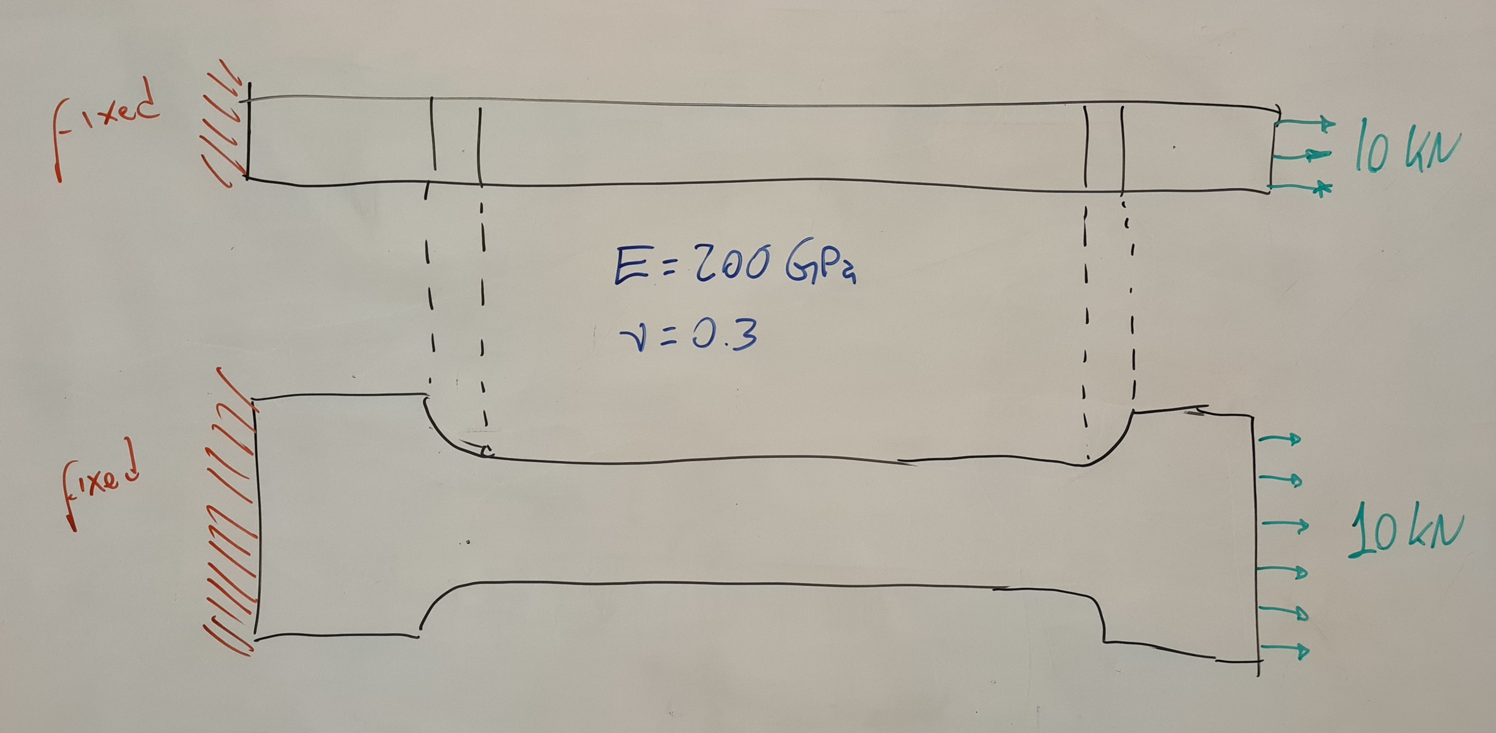
A tensile test specimen of nominal cross-sectional area A = 20~\text{mm} \times 5~\text{mm} = 100~\text{mm}^2 is fully fixed on one end (flat end face normal to the x axis at x<0, magenta surface not shown) and a tensile load of F_x = 10~\text{kN} is applied at the other end (flat end face at x>0, green surface). The Young modulus is E=200~\text{GPa} and the Poisson’s ratio is \nu=0.3.
Figure 1: Tensile test specimen CAD from CAEplex https://caeplex.com/p/41dd1 (rotate and zoom it).
2.1 Expected results
- Compute the displacement and stress distribution within the geometry. Create pictures of their distribution with a post-processing tool.
- Show that the specimen experiences elongation along the x axis and a mild contraction in y (and even milder in z).
- Check that the normal tension at the center of the specimen matches the theoretical solution \sigma_x = F_x/A
- Check that the reaction at the fixed end balances the external load \mathbf{F} applied at the opposite face.
- Show that there are stress concentrations at the heads of the coupon.
3 Geometry and mesh
Following the general idea of performing only one thing well (thoroughly discussed in the FeenoX Software Design Specification), and the particular Unix rules (sec. 6) of
- composition, and
- parsimony
the generation of the set of nodes and elements required to perform a mechanical computation using the finite element method is outside of FeenoX’ scope. That is to say,
The finite-element mesh is not a direct input of FeenoX. It has to be created and stored in a separate file which is then referred from the actual input file.
In the particular case of the tensile test problem, the geometry is given as a STEP file. It is meshed by Gmsh (or, following the rule of diversity, any other meshing tool which can write meshes in MSH format keeping information about physical groups).
A 3D CAD file consists of volumes, surfaces, edges and vertices. Each volume is defined by a set its boundary surfaces, each surface by a set of its boundary edges, and each edge by a set of its boundary vertices. Depending on the problem dimension, these geometrical entities will be linked to either material properties or boundary conditions:
| Problem dimension | Material properties | Boundary conditions |
|---|---|---|
| 3 | Volumes | Surfaces, edges and vertices |
| 2 | Surfaces | Edges and vertices |
| 1 | Edges | Vertices |
Even though mathematically speaking the whole boundary of the domain ought to have an associated boundary condition, depending on the type of physical problem being solved, some entities in the boundary might not need to have an explicit boundary condition. For instance, when solving a mechanical problem, those surfaces without an explicit condition are treated as “free” surfaces, i.e. free to deform with a traction identically zero without a prescribed displacement. For a thermal heat-conduction problem, free surfaces usually mean they are treated as adiabatic. In general, each case has to be checked with the documentation of the finite-element tool being used to solve the problem. In the case of FeenoX, we will walk through them togeteher.
The creation of a finite-element mesh involves basically four steps:
- reading the CAD file with the continuous domain of the problem,
- identifying the continuous volumes that will be linked to material properties,
- identifying the continuous surfaces, edges and vertices that will be linked to boundary conditions ,
- setting up meshing options, such as the elements’
- type: tetrahedra or hexahedra (there might be transition elements such as wedges, pyramids, etc. as well)
- order: linear or quadratic (higher-order elements are not currently supported in FeenoX)
- sizing: characteristic edge sizes, possible locally-refined
- quality: extra optimization steps to remove negative jacobians (in curved second-order elements) and improve overall mesh quality
- etc.
Since we are solving a mechanical problem with FeenoX, any surface (or edge or vertex) that does not have an explicit boundary condition will act as a free surface (homogeneous traction). Also, the problem asks for conditions on only two surfaces, namely the two longitudinal ends of the tensile test specimen so we have to identify only these two faces. Moreover, since there is only one volume in the CAD file we do not need to explicitly link it to material properties (as there is only one, the link is trivial and it is performed automatically by FeenoX as explained in the next section). But still, we need to identify it so as to have Gmsh to generate the bulk elements.
If you have not already, clone the FeenoX repository and
cdtodoc/tutorials/110-tensile-test. Make sure you havegitinstalled first.$ sudo apt-get install git [...] $ git clone https://github.com/seamplex/feenox/ Cloning into 'feenox'... remote: Enumerating objects: 8224, done. remote: Counting objects: 100% (1126/1126), done. remote: Compressing objects: 100% (567/567), done. remote: Total 8224 (delta 599), reused 959 (delta 528), pack-reused 7098 Receiving objects: 100% (8224/8224), 20.76 MiB | 17.25 MiB/s, done. Resolving deltas: 100% (5873/5873), done. $ cd feenox/doc/tutorials/110-tensile-test $In a shell capable of doing graphics, open the file
tensile-test-specimen.stepwith Gmsh:$ gmsh tensile-test-specimen.stepRotate the model until you see the whole 3D geometry and ask Gmsh to show the ids of the geometrical surfaces by going to
- Tools \rightarrow Options \rightarrow Geometry \rightarrow Surface labels
You should see something like this:
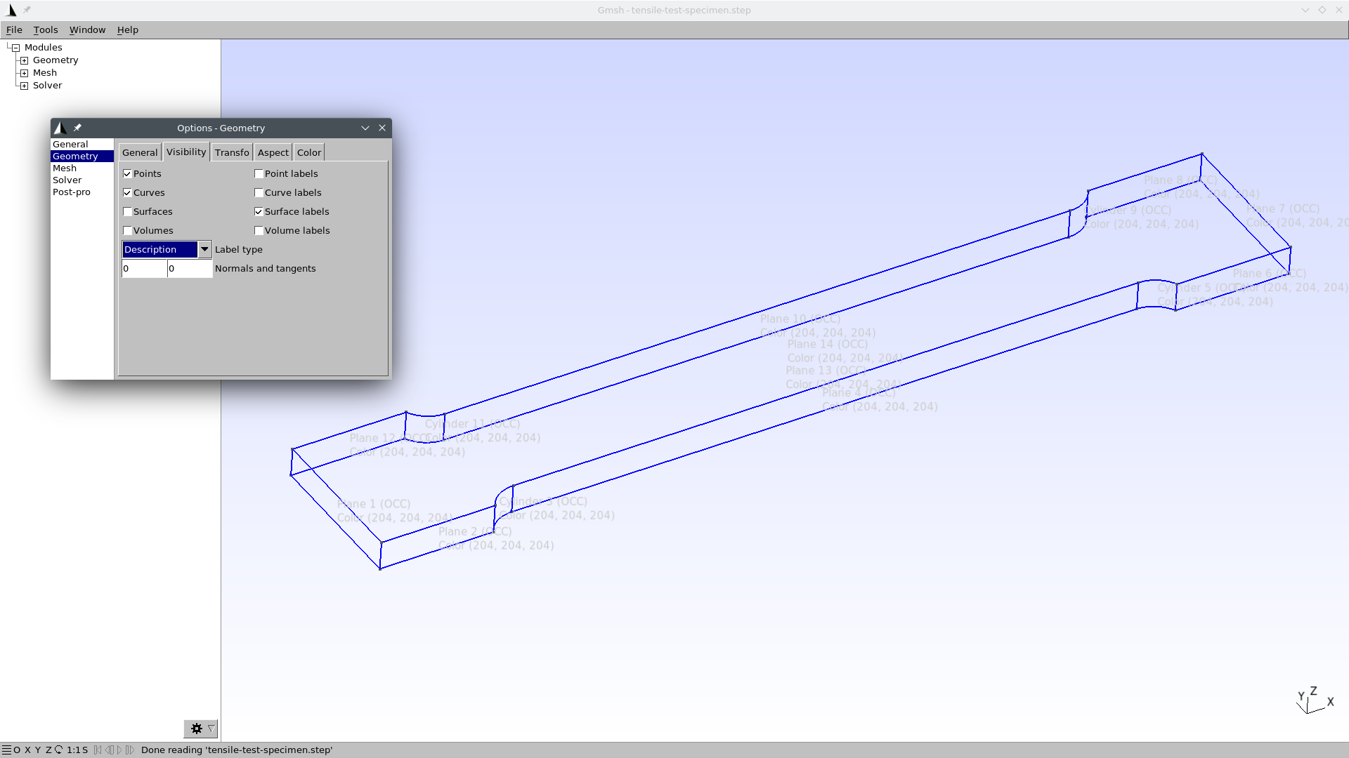
Note that the left-most (in the x axis) surface has an id of one and the right-most surface has an id of seven. That’s all we need to know about the CAD model, that the “left” surface is 1 in the STEP and that “right” is 7. You can close the Gmsh graphical window now.
Open your text editor (mine is Kate with syntax highlighting set to “C”) and create a file named
tensile-test.geowith the following content:// step #1: read the cad file (length units are millimeters) Merge "tensile-test-specimen.step"; // step #2: identify volumes // there's only one volume, the id is 1 and the name can be anything Physical Volume ("bulk") = {1}; // step #3: identify surfaces // the name between brackets will appear in the FeenoX input file in the BC keyword Physical Surface ("left") = {1}; // left face, to be fixed Physical Surface ("right") = {7}; // right face, will hold the load // step #4: Mesh.MeshSizeMax = 3; // set the max element size lc (in mm) Mesh.ElementOrder = 2; // ask for second-order tetrahedra Mesh.OptimizeNetgen = 1; // optimize linear elements Mesh.HighOrderOptimize = 3; // optimize quadratic elementsCall Gmsh from the shell passing
-3as the first parameter andtensile-test.geoas the second to create a three-dimensional mesh (that is what the-3means) namedtensile-test.msh(this step does not need to have a graphical terminal):$ gmsh -3 tensile-test.geo Info : Running 'gmsh -3 tensile-test.geo' [Gmsh 4.10.5, 1 node, max. 1 thread] Info : Started on Sat Sep 10 15:22:59 2022 Info : Reading 'tensile-test.geo'... Info : Reading 'tensile-test-specimen.step'... Info : - Label 'Shapes/ASSEMBLY/=>[0:1:1:2]/Pad' (3D) Info : - Color (0.8, 0.8, 0.8) (3D & Surfaces) Info : Done reading 'tensile-test-specimen.step' Info : Done reading 'tensile-test.geo' Info : Meshing 1D... Info : [ 0%] Meshing curve 1 (Line) Info : [ 10%] Meshing curve 2 (Line) Info : [ 10%] Meshing curve 3 (Line) [...] -----8<----- more output cut out -----8<----- [...] Info : Final volume mesh: worst distortion = 0.796943 (0 elements in ]0, 0.2]) Info : Done applying elastic analogy to high-order mesh (0.652083 s) Info : Done optimizing mesh (Wall 0.595085s, CPU 0.652091s) Info : 10754 nodes 8949 elements Info : Writing 'tensile-test.msh'... Info : Done writing 'tensile-test.msh' Info : Stopped on Sat Sep 10 15:23:01 2022 (From start: Wall 1.35632s, CPU 1.62598s) $If you don’t like Gmsh’ verbosity, you can change it with the command-line option
-v. I recommend you read its extensive documentation for further details.Now that the mesh file has been created, you can open it with the Gmsh GUI to check how it looks like.
$ gmsh tensile-test.mshBy default, Gmsh will show you something like this:
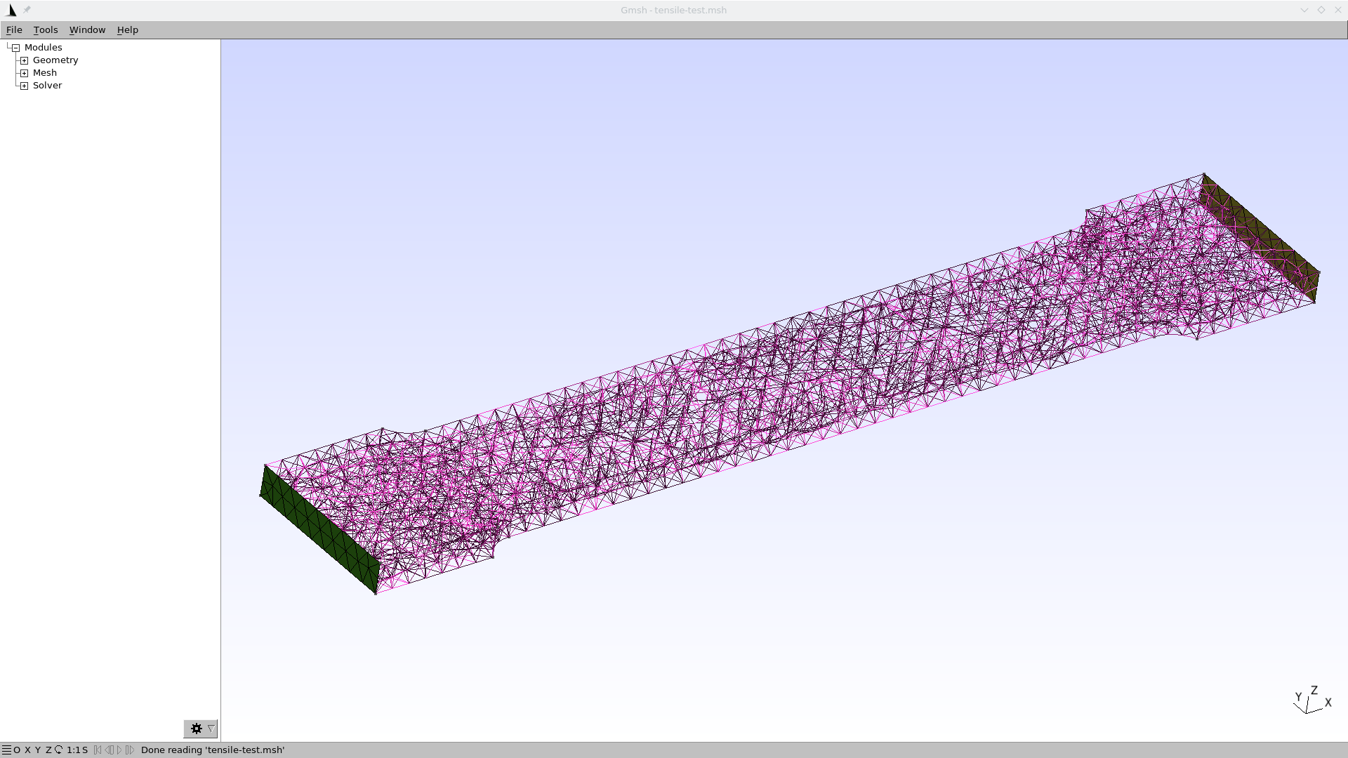
Here you can see that both end surfaces have “explicit” triangles while the rest of the surfaces seem to be hollow. This comes from the fact that we defined physical groups only for the two end faces and not for the rest of the faces—which is perfectly fine. We can ask for a nicer view by going to
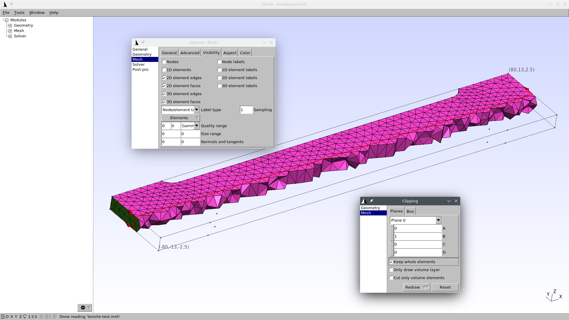
- Tools \rightarrow Options \rightarrow Mesh \rightarrow 3D element faces
We can then add a clipping plane to peek at the tetrahedra in the bulk of the specimen:
- Tools \rightarrow Clipping \rightarrow Mesh \rightarrow A=0, B=1, “Keep whole elements”
Now you should get
Feel free to close Gmsh now, we are done with it.
In general, multi-solid problems need to have different physical volumes in order for FeenoX to be able to set different mechanical properties. Even though this simple problem has a single solid and an explicit link is not needed, a physical volumetric group is needed in order for Gmsh to write the volumetric elements (i.e. tetrahedra) into the output MSH file (which is an input for FeenoX).
The usage of physical groups to define boundary conditions follows the rule of representation as it folds knowledge into data instead of focusing on algorithmically setting loads on individual nodes, which is a common practice among some finite-element solvers. The reason is that asking for nodal loads in the solver’s input file makes the programmer’s life easier but the user’s life harder. However, complicating things for a few developers only once but simplifying things for a lot of users during the lifespan of an engineering software tool is definitely a wise design choice.
This approach of using physical groups to set boundary conditions that refer to actual CAD faces means that the formulation of the problem being solved is completely determined from the continuous CAD geometry and does not depend on the details of the mesh. This allows for extensibility in at least two ways:
The mesh can be refined (or coarsened) arbitrarily, either by
- changing the value of
Mesh.MeshSizeMaxin the GEO file, - passing a refinement factor in Gmsh’s command-line option
-clscale, and/or - using one of the many ways of specifying mesh element sizes,
and then using it in FeenoX with exactly the same input file. There is no need to re-compute nodal loads nor to perform any other pre-processing step, providing simplicity. More advanced tutorials (and some examples such as this one) show how to perform parametric mesh convergence studies (and even optimization loops).
- changing the value of
A mesh with many physical groups can be used for many cases (say a tensile case first and a bending case later) where they set different boundary conditions on different sets of physical groups. This provides clarity.
4 FeenoX Input file
FeenoX reads a plain-text input file—which in turns also reads the mesh generated in the previous section—that defines the problem, asks FeenoX to solve it and writes whatever output is needed. See section “Interfaces” in the SDS for a thorough discussion of both inputs and outputs.
The input file is a syntactically-sweetened way to ask the computer to perform the actual computation (which is what computers do). This input file, as illustrated in the example below lives somewhere near the English language so a person can read through it from the top down to the bottom and more or less understand what is going on (rule of least surprise). The idea is that this input file should match as much as possible the definition of the problem as an engineer would cast it in a plain sheet of paper (or blackboard).
Yet in the extreme case that the complexity of the problem asks for, the input file could be machine-generated by a script or a macro (rule of generation). Or if the circumstances call for an actual graphical interface for properly processing (both pre and post) the problem, the input file could be created by a separate cooperating front-end such as CAEplex in fig. 1 above (rule of separation). In any case, the input files—both for Gmsh and for FeenoX—can be tracked with Git in order to increase traceability and repeatability of engineering computations. This is not true for most of the other FEA tools available today, particularly the ones that do not follow McIlroy’s recommendations above.
Given that the problem is relatively simple, following the rule of simplicity,
the input file tensile-test.fee ought to be
also simple. Other cases with more complexity might lead to more complex
input files.
Out of the full input file listed in sec. 1, the lines that actually ask FeenoX to perform the problem at hand are:
PROBLEM mechanical           # self-descriptive
READ_MESH tensile-test.msh   # lengths are in mm

# material properties, E and nu are "special" variables for the mechanical problem
E = 200e3   # [ MPa = N / mm^2 ]
nu = 0.3

# boundary conditions, fixed and Fx are "special" keywords for the mechanical problem
# the names "left" and "right" should match the physcal names in the .geo
BC left  fixed
BC right Fx=10e6  # [ N ]

# we can now solve the problem, after this keyword the results will be available for output
SOLVE_PROBLEM

# guess
WRITE_RESULTS FORMAT vtk
The details of why, how and what “FeenoX input files” look like is discussed in section 3.1 of the Software Design Specification. TL; DR: there are
- definitions (nouns), and
- instructions (verbs).
The first line is a definition (“problem” is a noun) that asks FeenoX to solve a mechanical problem. The second line is an instruction (“read” is a verb) that reads the mesh that we created in the previous step.
The next two lines are instructions that assign numerical values to
specially-named variables that hold the material properties using the
= instruction. In this case, since there is only one
material with homogeneous properties we can use the special scalar
variables E and nu to hold the Young modulus
and Poisson’s ratio respectively. For completeness, this is a quick
table about how to define material properties:
| Single material | Multi material | |
|---|---|---|
| Homogeneous | E = 200e3 |
E_name = 200e3 |
| Non-homogeneous | E(x,y,z) = 1000/(800-T(x,y,z)) |
E_name(x,y,z) = 1000/(800-T(x,y,z)) |
Since this is the first tutorial, it is expected that we have to
handle the simpler case, namely E=200e3 and
nu=0.3. Some further comments about these two lines:
Although we are “defining” material properties, the
=operator is actually and instruction that assigns the expression in the right-hand side to the variable in the left-hand side. The mechanical problem usesEandnuas special variables for homogeneous isotropic material properties. Modal also needrhofor density and thermal useskfor conductivity. If we were defining non-homogeneous properties instead, we would be defining a function of spaceE(x,y,z)that can be given by an algebraic expression as in the table above or by interpolating reading point-wise defined data from various sources. More details in further tutorials, or you can browse the examples like this or this one. Compare with the way of setting non-homogeneous properties in other FEA software.Mind the units! The mesh defines the location of nodes using a certain length unit, in this case millimeters. That means that the denominator of units of the Young modulus are millimeters squared. Now, if we use Newtons for the loads (wait until we discuss the boundary conditions below), that means that the numerator is Newton. Hence, E is expected to be in Mega Pascals = N \cdot mm^{-2}. It does not matter if you define first the units of stress for E and then the units of force and length or whatever order suits you. You have to be consistent.
The right hand side is expected to be an expression. So if \nu was numerically equal to one third, the line
nu = 1/3would be perfectly valid. In FeenoX, everything is an expression. Remember that (and compare with what you have to do to write algebraic expressions in other FEA software).
Note that this simple case where there is only one material, we do not have to “link” material properties to physical volume in the mesh. FeenoX is smart enough to figure it out by it own, need to tell it the obvious. Compare with other FEA software.
The next two lines set the boundary conditions:
# boundary conditions, fixed and Fx are "special" keywords for the mechanical problem
# the names "left" and "right" should match the physical names in the .geo
BC left  fixed
BC right Fx=10e3  # [ N ]
The keyword BC
tells FeenoX that it has
to set a boundary condition on the physical surface given by the second
word. This time we do need to give a physical surface name, since
nothing is obvious here. The type and value of the boundary condition is
defined by the remaining of the line:
- the “left” surface is fully
fixed, which is a shortcut foru=0,v=0andw=0. - the “right” surface has a total force in the x direction equal to one thousand Newtons
More complex settings like defining values individual degrees of freedom or multiple physical groups are possible with a slightly more complex syntax. As before, remember that everything is an expression so
BC right Fx=0.05*E # [ N ]is also perfectly valid, provided the units of the factor 0.05 make sense. Compare with how boundary conditions have to be set in other FEA software.
The final line contains the keyword SOLVE_PROBLEM
telling FeenoX that all
keywords needed to fully define the problem have been already given and
it can proceed to solve it. When executed, FeenoX will read all the
definitions and define whatever is needed to be defined. It will then
execute all the instructions in the order of appearance in the input
file, minding some basic conditional blocks. When it executes
SOLVE_PROBLEM, well, it solves the problem.
4.1 Outputs
The remaining part of the input file writes the five results that the problem formulation expects to be computed as required in sec. 2.1. Note (and compare with other FEA software) that the output in FeenoX is 100% defined by the user. If there are no output instructions, FeenoX will—following the Unix rule of silence—run silently. If the user wants to know something, she will have to ask FeenoX for an explicit output. The rationale behind this rule is that engineering time is far more expensive than computer time. Therefore, most of the time it makes much more sense to re-run a case that directly shows what one needs instead of having to manually browse through tons of numbers in order to find one single value. This last policy comes from really old design patterns dating from times when computer time was more expensive than people’s time. Again, compare with other FEA software.
4.1.1 Displacements and stresses
# 1. a VTK file to be post-processed in ParaView with
# a. the displacements [u,v,w] as a vector
# b. the von Mises stress sigma as a scalar
# c. the six components of the stress tensor as six scalars
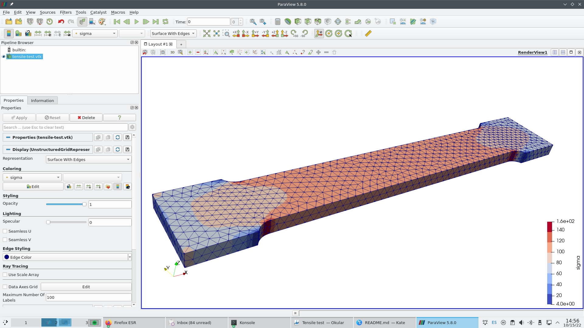
WRITE_MESH tensile-test.vtk VECTOR u v w sigma sigmax sigmay sigmaz tauxy tauyz tauzx
PRINT "1. post-processing view written in tensile-test.vtk"The instruction WRITE_MESH
asks FeenoX to write a
file for post-processing. Here, we want to write a file named
tensile-test.vtk containing a vector with the three
displacements [u,v,w], then the von
Mises stress \sigma and finally the six
components of the stress tensor.
4.1.2 Show elongation and contraction
# 2. the displacement vector at the center of the specimen
PRINT "2. displacement in x at origin:   " u(0,0,0)   "[ mm ]"
PRINT "   displacement in y at (0,10,0): " v(0,10,0)  "[ mm ]"
PRINT "   displacement in z at (0,0,2.5):" w(0,0,2.5) "[ mm ]"
The displacement field can be accessed as three scalar functions of
space u(x,y,z), v(x,y,z) and w(x,y,z). These functions can be evaluated at
any arbitrary point in space, and that is what these PRINT
instructions do.
4.1.3 Check normal tension at center
# 3. the principal stresses at the center
PRINT "3. principal stresses at origin: " %.4f sigma1(0,0,0) sigma2(0,0,0) sigma3(0,0,0) "[ MPa ]"
Same thing happens to the principal stresses \sigma_1, \sigma_2 and \sigma_3.
4.1.4 Check reactions
# 4. the reaction at the left surface
COMPUTE_REACTION left  RESULT R_left
PRINT "4. reaction at left surface: " R_left "[ N ]"
The COMPUTE_REACTION
keyword takes a physical group as the first parameter and stores the
result in either the scalar or vector given after RESULT.
In this case, it is a vector whose three elements are printed in the
same line.
4.1.5 Show stress concentrations
# 5. stress concentrations at a sharp edge
PRINT "5. stress concentrations at x=55, y=10, z=2.5 mm"
PRINT "von Mises stress:" sigma(55,10,2.5) "[ MPa ]"
PRINT "Tresca    stress:" sigma1(55,10,2.5)-sigma3(55,10,2.5) "[ MPa ]"
PRINT "stress tensor:"
PRINT %.1f sigmax(55,10,2.5) tauxy(55,10,2.5)  tauzx(55,10,2.5)
PRINT %.1f tauxy(55,10,2.5)  sigmay(55,10,2.5) tauyz(55,10,2.5)
PRINT %.1f tauzx(55,10,2.5)  tauyz(55,10,2.5)  sigmaz(55,10,2.5)
A couple of PRINTs.
Note that FeenoX does not
have a Tresca stress function, but it can be easily computed as \sigma_1-\sigma_3. Recall that “everything is
an expression.”
4.2 Notes
Some notes summarizing the section:
The FeenoX input file is clean as a whistle:
- It is syntactically sugared by using English-like keywords.
- Nouns are definitions and verbs are instructions.
- Simple problems need simple inputs.
- Simple things should be simple, complex things should be possible.
- Whenever a numerical value is needed an expression can be given (i.e. “everything is an expression.”)
- The input file should match as much as possible the paper (or blackboard) formulation of the problem.
- Input files are distributed version control-friendly.
See a more detailed description (and discussion) about the input in section 3 of the Software Design Specification.
The mesh
tensile-test.mshfile is the output of Gmsh when invoked with the inputtensile-test.geoabove. It can be either version 4.1 or 2.2. It is not part of FeenoX the input file, but referred to by the file name. This allows the input file to be tracked by Git (or any other DVCS).The mechanical properties, namely the Young modulus E and the Poisson’s ratio \nu are uniform in space. Therefore, they can be simply set using special variables
Eandnu.Boundary conditions are set by referring to the physical surfaces defined in the mesh. The keyword
fixedis a shortcut for setting the individual displacements in each directionu=0,v=0andw=0.An explicit location within the logical flow of the input file hast to be given where FeenoX ought to actually solve the problem with the keyword
SOLVE_PROBLEM. It should be after defining the material properties and the boundary conditions and before computing secondary results (such as the reactions) and asking for outputs.The reaction in the physical group “left” is computed after the problem is solved (i.e. after
SOLVE_PROBLEM) and the result is stored in a vector namedR_leftof size three. There is nothing special about the nameR_left, it could have been any other valid identifier name.A post-processing output file in format VTK is created, containing:
- The displacement vector \mathbf{u}=[u,v,w] as a three-dimensional vector field
- The von Mises stress
sigma(\sigma) as an scalar field - The six components of the stress tensor
sigmax,sigmay,sigmaz,tauxy,tauyzandtauzx(\sigma_x, \sigma_x, \sigma_x, \tau_{xy}, \tau_{yz}, \tau_{zx} respectively) as six scalar fields
Some of the asked results are printed to the terminal (i.e. the standard output). Note that
- The actual output (including post-processing files) is 100% defined by the user, and
- If no output instructions are given in the input file
(
PRINT,WRITE_MESH, etc.) then no output will be obtained.
Not only do these two facts follow the rule of silence but they also embrace the rule of economy: the time needed for the user to find and process a single result in a soup of megabytes of a cluttered output file far outweighs the cost of running a computation from scratch with the needed result as the only output.
The principal stresses \sigma_1, \sigma_2 and \sigma_3 are evaluated at the origin. There is no need to have an actual node at \mathbf{x}=(0,0,0) since FeenoX can evaluate functions at any arbitrary point.
5 Execution
Opening a terminal and calling both Gmsh and FeenoX in sequence should go as smooth (and as fast) as follows.
Here is a static mimic of a 12-second terminal session:
$ gmsh -3 tensile-test.geo
Info    : Running 'gmsh -3 tensile-test.geo' [Gmsh 4.10.5, 1 node, max. 1 thread]
Info    : Started on Sat Oct  1 15:43:13 2022
Info    : Reading 'tensile-test.geo'...
Info    : Reading 'tensile-test-specimen.step'...
Info    :  - Label 'Shapes/ASSEMBLY/=>[0:1:1:2]/Pad' (3D)
Info    :  - Color (0.8, 0.8, 0.8) (3D & Surfaces)
Info    : Done reading 'tensile-test-specimen.step'
Info    : Done reading 'tensile-test.geo'
Info    : Meshing 1D...
Info    : [  0%] Meshing curve 1 (Line)
Info    : [ 10%] Meshing curve 2 (Line)
[...]
Info    : Done optimizing mesh (Wall 0.624045s, CPU 0.675089s)
Info    : 10754 nodes 8949 elements
Info    : Writing 'tensile-test.msh'...
Info    : Done writing 'tensile-test.msh'
Info    : Stopped on Sat Oct  1 15:43:15 2022 (From start: Wall 1.47622s, CPU 1.64583s)
$ feenox tensile-test.fee
1. post-processing view written in tensile-test.vtk
2. displacement in x at origin:         0.0376532       [ mm ]
   displacement in y at (0,10,0):       -0.00149662     [ mm ]
   displacement in z at (0,0,2.5):      -0.000375989    [ mm ]
3. principal stresses at origin:        99.9998 0.0002  -0.0000 [ MPa ]
4. reaction at left surface:    -10000  -0.000441991    -0.000318119    [ N ]
5. stress concentrations at x=55, y=10, z=2.5 mm
von Mises stress:       138.329 [ MPa ]
Tresca    stress:       138.917 [ MPa ]
stress tensor:
138.5   9.8     -2.1
9.8     2.1     -0.5
-2.1    -0.5    0.5
$
You can now open ParaView:
$ paraview tensile-test.vtkCongratulations! You just finished your first FeenoX tutorial!
Keep in mind this was a very detailed tutorial where we digged into a lot of subtle details. Forthcoming tutorials will not be as detailed as this one.
The problem was selected to be very simple. Any actual industrial application will need further discussions, such as
- The left face cannot be really fully fixed in a tensile test machine.
- There are other boundary conditions that better describe the actual physics.
- If we wanted to understand what happens in a pure tensile case we would need to have another type of boundary condition in the left face.
- The material properties are assumed to be uniform and linear. A thorough discussion of the application of these two assumptions have to be given before any actual application.
Please take some minutes to dig further down into the philosophy of what you just achieved.
6 Unix philosophy*
This section is optional so you can skip it. Nevertheless, it important that you read this section at least one.
FeenoX’ cloud-first design and implementation is largely based on the Unix philosophy, as introduced in Eric Raymond’s seminal book The Art of Unix Programming. A quotation from such seminal book helps to illustrate this idea:
Doug McIlroy, the inventor of Unix pipes and one of the founders of the Unix tradition, had this to say at the time:
Make each program do one thing well. To do a new job, build afresh rather than complicate old programs by adding new features.
Expect the output of every program to become the input to another, as yet unknown, program. Don’t clutter output with extraneous information. Avoid stringently columnar or binary input formats. Don’t insist on interactive input.
[…]
He later summarized it this way (quoted in “A Quarter Century of Unix” in 1994):
- This is the Unix philosophy: Write programs that do one thing and do it well. Write programs to work together. Write programs to handle text streams, because that is a universal interface.
Keep in mind that even though the quotes above and many FEA programs that are still mainstream today date both from the early 1970s, fifty years later they still
- Do not make just only one thing well.
- Do complicate old programs by adding new features.
- Do not expect the their output to become the input to another.
- Do clutter output with extraneous information.
- Do use stringently columnar and/or binary input (and output!) formats.
- Do insist on interactive output.
A further note is that not only is FeenoX both free and open-source software but it also is designed to connect and to work with (rule of composition) other free and open source software, like
and many others, including of course the operating system GNU/Linux.
Heads up: it is extremely important to note here that
the adjective “free” in the expression “free software” refers to freedom and not to price. A better wording would be “libre software” instead. When we say “free software” we mean “free” as in “free speech” not as in “free beer.” The difference will be made clear throughout the tutorial. In what follows, we use “gratis” or “for a fee” when referring to price and “free” and “privative” (because it privates users from their freedom) or “non-free” when referring to freedom.
“free software” does not mean “open source.” The two terms are related but not equal, having different technical and ethical meanings with different roots and rationales for each one. There are books and discussions online about the matter. The important thing to remember here is that FeenoX is both free and open source under the terms of GNU General Public License version 3 or, at the user convenience, any later version. The opposite is of “open source” is “closed source.” Note that a closed-source piece of software is privative by definition, but an open-source piece of software can be either free (as most open-source software is) or non-free (as a tiny fraction is).
the importance of FeenoX (and in general any engineering-related tool) being free (it is GPLv3+) and open source (its source tree can be cloned from Github) is way more profound than the basic fact you do not have to pay a software license. The most important issue of FeenoX being open source is that anyone can
- see,
- analyze, and eventually
- understand
what equations are being solved and how they are being solved with a digital computer. The most important issue of FeenoX being free software, besides the three pints above, is that anyone can modify it to suit their needs and then share those modifications. Of course most people do not know how to see, analyze, understand and/or modify computational source code. But the main key is that these people have the freedom to ask somebody else to do it for them, either gratis or for a fee. This is not the case for other non-free (wrongly called “commercial”) engineering tools, where users do not have the freedom to see what and how the equations are being solved, let alone asking a third party to review them.
On the other hand, even though it is true that FeenoX can be executed by anyone without paying any royalty to the owner of the copyright, that does not mean that its usage is completely gratis. These issues still hold:
- Downloading and executing the tool might incur in expenses such as electricity consumption, network connections, storage capacity, computing power, etc.
- Even though the tool is freely distributed under the GPLv3+, people distributing it can charge a fee for the distribution. It is not illegal to sell free software for a fee. It is illegal to prevent other people from distributing it gratis and to prevent other people from accessing the source code, though.
- There can be services that provide the execution of the tool in the cloud (i.e. somebody else’s computer) for a fee (e.g. CAEplex).
- The code does have a copyright owner, which is the original author of FeenoX. Yet, instead of using these rights to take freedom away from its users, they are used to make nobody can take it away by using the copyleft licensing mechanism.
- There might be application cases for which the tool as it is might be limited or inadequate. As already discussed, it is possible (i.e. anybody has the freedom) to hire someone (possibly the original author of the code) to modify FeenoX in order to add features or functionalities in such a way to allow for the adequate application of the tool. These kind of works might involve a development fee.
In particular, this tutorial has been created from scratch using free and open source software only (Markdown converted to PDF and HTML with Pandoc using Kate as the main editor). Even the terminal recorder used to show the actual execution is GPLv3.
Following the Unix philosophy, FeenoX also makes use of high-quality free and open source mathematical libraries which contain numerical methods designed by mathematicians and programmed by professional programmers instead of hard-coding ad-hoc mathematical algorithms. In particular, it uses
- GNU Scientific Library
- PETSc (and all its respective dependencies)
- SLEPc
- kdtree
- uthash
This way, FeenoX bounds its scope to doing only one thing and to doing it well: namely, to build and solve finite-element formulations of partial differential equations instead of implementing numerical methods to solve the discretized equations. And it does so on high grounds, both
ethical: since it is free software, all users can
- run,
- share,
- modify, and/or
- re-share their modifications.
If a user cannot read or write code to either
- check that FeenoX solves the right equations right (i.e. to perform independent verification and validation), and/or
- to modify FeenoX to suit their needs,
at least they has the freedom to hire someone to do it for her, and
technological: since it is open source, advanced users can detect and correct bugs and even improve the algorithms. Given enough eyeballs, all bugs are shallow.
Check out the programming and contributing section of the FeenoX documentation for further details regarding
- FeenoX’s roadmap
- Programming languages
- Coding styles and guidelines
- Rules of conduct
- Related tools
- etc.
A final comment is that FeenoX is designed to work as an engineering “transfer function” between one (or more) input files and zero (or more) output files (which might include the terminal):
                             +------------+
 mesh (*.msh)  }             |            |             { terminal
 input (*.fee) } input ----> |   FeenoX   |----> output { data files
 data file     }             |            |             { post (vtk/msh)
                             +------------+
In computer-science, this transfer-function-like workflow is called a filter or pipe. Indeed, we already quoted Doug McIlroy who invented Unix pipelines. When solving a finite-element problem, FeenoX thus needs two files:
- A FeenoX input file (discussed in sec. 4)
- A mesh file (discussed in sec. 3)
Depending on the expected results (sec. 2.1) there might be zero (i.e. rule of silence) or more outputs, such as